CS 332 Assignment 3 Due: Friday, October 29

This assignment contains three problems on the analysis of visual motion. In the first problem, you will implement a stategy to track the moving cars in a video of an aerial view of a traffic scene, and visualize the results. In the second problem, you will complete a function to compute the perpendicular components of motion and analyze the results of computing a 2D image velocity field from these components. In the final problem, you will explore the 2D image velocity field that is generated by the motion of an observer relative to a stationary scene, and the computation of the observer's heading from this velocity field. You do not need to write any code for the third problem. The code files for all three problems are stored in a folder named motion that you can download through this motion zip link. (This link is also posted on the course schedule page and the motion folder is also stored in the /home/cs332/download/ directory on the CS file server.)

Submission details: Submit an electronic copy of your code files for Problems 1 and 2 by dragging the tracking and motionVF subfolders from the motion folder into the cs332/drop subdirectory in your account on the CS file server. The code for these problems can be completed collaboratively with your partner(s), but each of you should drop a copy of this folder into your own account on the file server. Be sure to document any code that you write. For your answers to the questions in Problem 3, create a shared Google doc with your partner(s). You can then submit this work by sharing the Google doc with me — please give me Edit privileges to that I can provide feedback directly in the Google doc.

Problem 1 (50 points): Tracking Moving Objects

The tracking subfolder inside the motion folder contains a video file named sequence.mpg that was obtained from a static camera mounted on a building high above an intersection. The first image frame of the video is shown below:

While you are working on this problem, set the Current Folder in MATLAB to the tracking subfolder. The code file named getVideoImages.m contains a script that reads the video file into MATLAB, shows the movie in a figure window, extracts three images from the file (frames 1, 5, and 9 of the video), displays the first image using imtool, and shows a simple movie of the three extracted images, cycling back and forth five times through the images. We will go over the getVideoImages.m code file in class, which uses the concept of a structure in MATLAB, and the built-in functions VideoReader, struct, read, and movie.

Most of the visual scene is stationary, but there are a few moving cars and pedestrians, and a changing clock in the bottom right corner. Your task is to detect the moving cars and determine their movement over the three image frames stored in the variables im1, im2, and im3. (The clock has been removed from these three images.) To solve this problem, you will use a strategy that takes advantage of the fact that most of the scene is stationary, so changes in the images over time occur mainly in the vicinity of moving objects. The image regions that are likely to contain the moving cars are fairly large regions that are changing over time.

Create a new script named trackCars.m in the tracking subfolder, to place your code to analyze and display the movement of the cars across the three images provided. (You are welcome to define separate functions for subtasks, but this is not necessary.) Implement a solution strategy incorporating the following steps:

• For each pair of consecutive images (i.e. the pair im1 and im2, and the pair im2 and im3), find image locations where many pixels within a neighborhood around the location have a large change in brightness between the two images. Some trial-and-error exploration will be needed to determine a reasonable neighborhood size, an appropriate threshold on the brightness change, and a good value for the fraction of changing pixels in the neighborhood that is used to decide that the region may contain a moving car
• Find large connected regions of locations where brightness is changing between the two images — these regions are likely to correspond to individual cars or parts of cars (the built-in function bwlabel can be helpful here)
• Determine the approximate center of each large connected region, corresponding to the rough location of each car (the built-in function regionprops can be helpful here)
• Given the car locations identified using the image pair im1 and im2, and the car locations identified using the image pair im2 and im3, match up the locations of the cars at these two moments in time, assuming that a car region at one moment moves to the closest car region at the next moment
• Display the results of your analysis. In the solutions that I demonstrated in class, subplot was used to create one figure window with three display areas showing the first image im1 and the large connected regions obtained from analyzing the two image pairs, with superimposed red dots shown at the center of each region. A second figure window displayed im1 with superimposed red lines showing the movement of each car over time.

Hints: The file codeTips.m in the tracking folder provides simple examples of some helpful coding strategies, including examples that use the built-in bwlabel and regionprops functions, access information stored in a vector of structures, and superimpose graphics (using the built-in plot and scatter functions), on an image that is displayed in a figure window.

Be sure to comment your code so that your solution strategy is clear! (You are welcome to use a different strategy than the one outlined above.)

Problem 2 (25 points): Computing a Velocity Field

In class, we described an algorithm to compute 2-D velocity from the perpendicular components of motion, assuming that velocity is constant over extended regions in the image. Let (Vx,Vy) denote the 2D velocity, (uxi,uyi) denote the unit vector in the direction of the gradient (i.e. perpendicular to an edge) at the ith image location, and v⊥i denote the perpendicular component of velocity at this location. In principle, from measurements of uxi, uyi and v⊥i at two locations, we can compute Vx and Vy by solving the following two linear equations:

   Vx ux1 + Vy uy1 = v⊥1
   Vx ux2 + Vy uy2 = v⊥2

In practice, a better estimate of (Vx,Vy) can be obtained by integrating information from many locations and finding values for Vx and Vy that best fit a large number of measurements of the perpendicular components of motion. The function computeVelocity, which is already defined for you, implements this strategy. Details of this solution are described in an Appendix to this problem.

To begin, set the Current Folder in MATLAB to the motionVF subfolder in the motion folder. The function getMotionComps, which you will complete, computes the initial perpendicular components of motion. This function has three inputs - the first two are matrices containing the results of convolving two images with a Laplacian-of-Gaussian function. It is assumed that there are small movements between the original images. The third input to getMotionComps is a limit on the expected magnitude of the perpendicular components of motion (assume that a value larger than this limit is erroneous and should not be recorded). This function has three outputs that are matrices containing values of ux, uy and v⊥. These quantities are computed only at the locations of zero-crossings of the second input convolution. At locations that do not correspond to zero-crossings, the value 0 is stored in the output matrices. The function definition contains ??? in several places where you should insert a simple MATLAB expression to complete the code statements. See the comments for instructions on completing each statement.

The motionTest.m script file contains two examples for testing your getMotionComps function. The first example uses images of a circle translating down and to the right. The expected results displayed for this example will be shown in class. The second example, which is initially in comments, uses a collage of four images of past Red Sox players, where each subimage has a different motion, as shown by the red arrows on the image below:

   

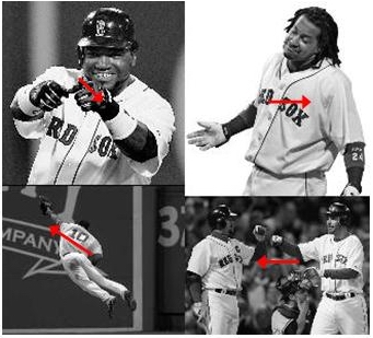
Big Papi (upper left) is shifting down and to the right, Manny (upper right) is shifting right, Varitek and Lowell (lower right) are shifting left, and Coco Crisp (lower left) is leaping up and to the left after a fly ball. For both examples, the velocities computed by the computeVelocity function are displayed by the displayV function in the motion folder, which uses the built-in quiver function to display arrows. Your results for the Red Sox image will roughly reflect the correct velocities within the four different regions of the image, but there will be significant errors in some places. Add comments to the motionTest.m script that answer the following questions: (1) where do most of the errors in the results occur? (2) why might you expect errors in these regions? Finally, the results will vary with the size of the neighborhood used to integrate measurements of the perpendicular components of motion. (3) what are possible advantages or disadvantages of using a larger or smaller neighborhood size for the computation of image velocity?

Appendix to Problem 2: Computing the Velocity Field in Practice

It was noted earlier that in principle, we can compute Vx and Vy by solving two equations of the form shown below, but in practice, a better estimate can be obtained by integrating information from many locations and finding values for Vx and Vy that best fit a large number of measurements of the perpendicular components of motion. Because of error in the image measurements, it is not possible to find values for Vx and Vy that exactly satisfy a large number of equations of the form:

   Vx uxi + Vy uyi = v⊥i

Instead, we compute Vx and Vy that minimize the difference between the left- and right-hand sides of the above equation. In particular, we compute a velocity (Vx,Vy) that minimizes the following expression:

   ∑[Vx uxi + Vy uyi - v⊥i]2

where ∑ denotes summation over all locations i. To minimize this expression, we compute the derivative of the above sum with respect to each of the two parameters Vx and Vy, and set these derivatives to zero. This analysis yields two linear equations in the two unknowns Vx and Vy:

   a1 Vx + b1 Vy = c1          a2 Vx + b2 Vy = c2

where

   a1 = ∑uxi2    b1 = a2 = ∑uxiuyi    b2 = ∑uyi2    c1 = ∑v⊥iuxi    c2 = ∑v⊥iuyi

The solution to these equations is given below, and implemented in the computeVelocity function:

   Vx = (c1b2 - b1c2)/(a1b2 - a2b1)          Vy = (a1c2 - a2c1)/(a1b2 - a2b1)

Problem 3 (25 points): Observer Motion

In this problem, you will explore the 2D image velocity field that is generated by the motion of an observer relative to a stationary scene, and the computation of the observer's heading from this velocity field. You do not need to write any code for this problem. You will be working with a MATLAB program that has a graphical user interface as shown below:

   

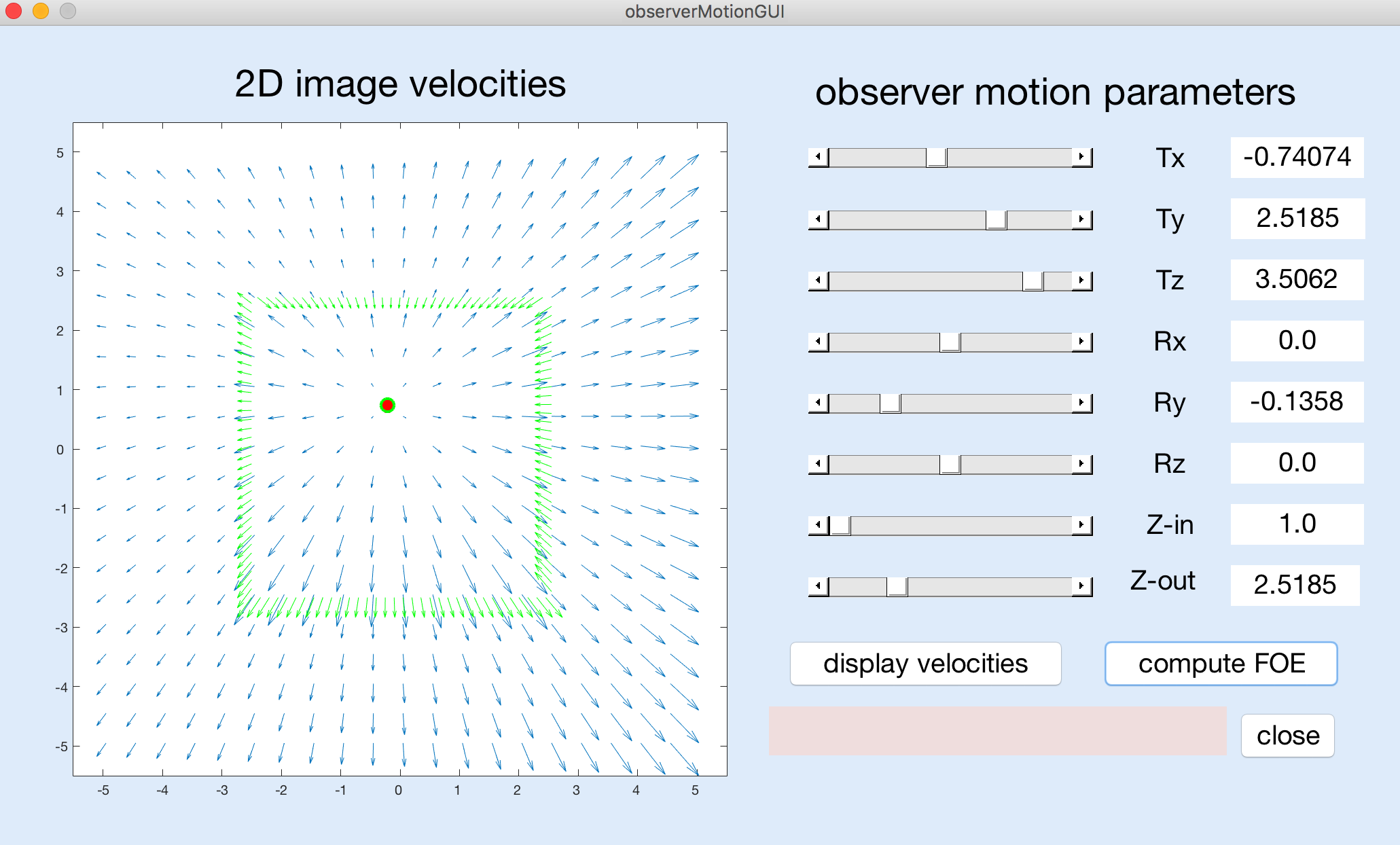
To begin, set the Current Folder in MATLAB to the observerMotion subfolder in the motion folder. To run the GUI program, just enter observerMotionGUI in the MATLAB command window. When you are done, click on the close button on the GUI display to terminate the program.

The GUI has six sliders that you can use to adjust the parameters of movement of the observer — the observer's translation in the x,y,z directions (denoted by Tx,Ty,Tz) and their rotation about the three coordinate axes (denoted by Rx,Ry,Rz). Each parameter has a different range of possible values that are controlled by the sliders and displayed along the right column of the GUI, e.g. Tx and Ty range from -6 to +6, Tz ranges from 0 to 4, Rx and Ry range from -0.25 to +0.25, and Rz ranges from -0.5 to +0.5. The 3D scene consists of a square surface in the center of the field of view whose depth is specified by Z-in that can range from 1 to 2, surrounded by a surface whose depth is specified by Z-out that can range from 2 to 4.

After setting the motion and depth parameters to a set of desired values using the sliders, you can click on the "display velocities" button to view the resulting velocity field, over a limited field of view defined by coordinates ranging from -5 to +5 in the horizontal and vertical directions. The coordinates (0,0) represent the center of the visual field corresponding to the observer's direction of gaze. If the true focus of expansion (FOE), indicating the observer's heading point, is located within this field of view, a red dot will be displayed at this location. Otherwise, the message "true FOE out of bounds" will appear in the pink message box near the lower right corner of the GUI.

After displaying the velocity field, you can click on the "compute FOE" button. The program runs an algorithm for computing the observer's heading that is based on the detection of significant changes in image velocity, as suggested by Longuet-Higgins and Prazdny. This algorithm first computes the differences in velocity between nearby locations in the image, and then combines the directions of large velocity differences to compute the FOE by finding the location that best captures the intersection between these directions. Large velocity differences will be found along the border of the inner square surface when there is a significant change in depth across the border. The velocity difference vectors will be displayed in green, superimposed on the image velocity field, with a green circle at the location of the computed FOE, as shown in the above figure. If the computed FOE is located outside the limited field of view that is shown in the display, the message "computed FOE out of bounds" will appear in the pink message box. If no large velocity differences are found that can be used to compute the FOE, the message "no large velocity differences" will appear in the message box.

In the exercises below, when I indicate that parameters should be set to particular values, use the associated sliders to reach values that are close to the desired values — they do not need to be exact. Note that the overall size of the graphing window changes slightly when showing the velocity field on its own ("display velocities" button) vs. showing the velocity field with the computed FOE and velocity difference vectors superimposed ("compute FOE" button) — when relevant, pay close attention to the actual x,y coordinates on the axes.

(1) Observe the velocity field obtained for each motion parameter on its own. First be sure that Z-in is set to 1 and Z-out is set to 2 (their initial values). Then set five of the six motion parameters to 0 (or close to 0) and view the velocity field obtained when the sixth parameter is set to each of its two extreme values (for Tz, use 4 and a small non-zero value). For each parameter, what is the overall pattern of image motion, and are there significant changes in velocity around the border of the central square? Which parameter(s) yield(s) a computable FOE in the field of view? Why is it not possible to compute an FOE for some motion parameters?

(2) In class, we noted that depth changes in the scene are needed to recover heading correctly. Set the five parameters Tx, Ty, Rx, Ry, and Rz to 0, and set Tz to 4. Then adjust the relative depth of the two surfaces. First set both Z-in and Z-out to 2. Can an FOE be computed in this case? Slowly change one of the two depths (either slowly decrease Z-in or slowly increase Z-out). How much change in depth is needed to compute the FOE in this case?

(3) This question further probes the need for depth changes. Again set both Z-in and Z-out to 2. Then examine the following two scenarios:

    (a) Ty = Rx = Ry = Rz = 0 and Tx = 6, Tz = 1.5

    (b) Same parameters as in (a) except that Ry = -0.25

What are the coordinates of the true FOE in each case? You'll observe that in both cases, the FOE cannot be computed because there are "no large velocity differences." In case (a) the observer is only translating and the overall velocity field expands outwards from the true FOE. This expanding pattern on its own could be used to infer the observer's heading, even in the absence of velocity differences due to depth changes in the scene. In case (b), suppose you searched for a center of expansion of the velocity field, where might you find such a point, and would it correspond to the observer's true heading point (true FOE)? How do the results in both cases change when you now introduce a depth change, i.e. set Z-in to 1 and set Z-out to 2?