CS 332 Assignment 2 Due: Wednesday, October 13

The first problem on this assignment considers stereo projection geometry and an additional constraint used in some stereo correspondence algorithms, known as the ordering constraint. The next two problems explore two methods for solving the stereo correspondence problem, a region based algorithm that uses the sum of absolute differences as a measure of similarity between regions of the left and right images, and the multi-resolution stereo algorithm proposed by Marr, Poggio, and Grimson. The final problem considers how key aspects of these two algorithms could be combined. The code files and images needed for Problem 2 are stored in a folder named stereo that you can download through this stereo zip link. (This link is also posted on the course schedule page and the stereo folder is also stored in the /home/cs332/download/ directory on the CS file server.)

Submission details: Submit an electronic copy of your code files for Problem 2 by dragging your stereo folder into the cs332/drop subdirectory in your account on the CS file server. The code for this problem should be completed collaboratively with your partner, but each of you should drop a copy of this folder into your own account on the file server. Be sure to document any code that you write. For your analysis of the simulation results in Problem 2 and your answers for Problems 1, 3, and 4, create a shared Google doc with your partner. For tasks involving diagrams, images from this document can be saved and inserted into slides and annotated, or a hardcopy could be annotated by hand and captured with a cell phone and inserted into the document. (Please let me know if you need help with this.) You can then submit this work by sharing the Google doc with me — please give me Edit privileges to that I can provide feedback directly in the Google doc.

Problem 1 (10 points): Stereo Projection and the Ordering Constraint

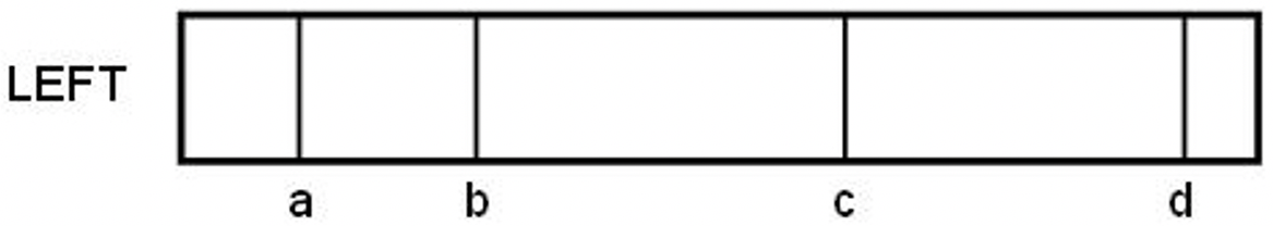
An additional constraint that is sometimes used in stereo correspondence algorithms is the ordering constraint. This constraint is derived from the fact that the horizontal order in which multiple corresponding features appear in the left and right images is typically the same in both views. Suppose, for example, there are four features in the left image, labeled a,b,c,d, in order of their appearance from left to right in the left image:

 

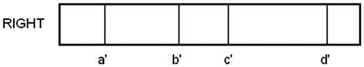
Let a',b',c',d' denote the corresponding features in the right image. The ordering constraint states that these matching features must occur in the right image in the same order a',b',c',d' from left to right, as shown here:

The following placement of corresponding features in the left and right images illustrates an example that violates the ordering constraint:

 

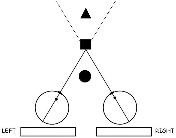
There are valid physical situations that violate the ordering constraint. One example occurs when objects are placed along a line in depth, as shown in the bird's eye view below. On this picture, first indicate where the projections of the circle, square, and triangle-shaped objects appear at the back of the left and right eyes, and sketch their approximate positions in the two image slices placed below the eyes. Assume that the eyes are focused on a point on the front surface of the square, as shown. In your diagram, clearly distinguish the circle, square, and triangle in some way. Then color in the region of 3D space in this bird's eye view that includes all possible positions of the circle that will result in stereo images of the square and circle together that violate the ordering constraint (i.e. the square and circle appear in opposite orders in the left and right images). To answer this question fully, first color the region within which the circle can be placed, so that it appears to the left of the square in the left image and to the right of the square in the right image. Then color the region where the circle can be placed so that it appears to the right of the square in the left image and to the left of the square in the right image. The combination of these two regions is sometimes referred to as the forbidden zone in the stereo literature.

 

Problem 2 (60 points): Exploring a Region-Based Stereo Algorithm

Before starting the computer work for this problem, set the Current Folder in MATLAB to the stereo folder, and add the edges subfolder (a copy of the same folder used in Assignment 1) to the MATLAB search path. For this problem, submit any code files that you wrote from scratch or modified, and answers to all the questions here.

Part a: Complete the compStereo function

The compStereo.m code file in the stereo folder provides some initial code for a function that implements a simple region based stereo correspondence algorithm. In the first part of this problem, you will complete the definition of the compStereo function following the outline described in the Stereo Correspondence video. A slightly modified outline is shown below:

For each location in the left image, stereo disparity should be computed by finding a patch in the right image at the same height and within a specified horizontal distance, which minimizes the sum of absolute differences between the right image patch and a patch of the same size centered on the left image location. The function should record both the best disparity at each location and the measure of the sum of absolute differences that was obtained for this best disparity, and return these values in two matrices. There should be a region around the perimeter of the image where no disparity values are computed. Carefully examine the initial code and comments to understand how the various input parameters are defined and the creation of initial variables.

Part b: Testing and enhancing the compStereo function

The stereoScript.m file contains code to run an example of stereo processing for a visual scene containing a variety of objects at different depths. The left and right images are first convolved with a Laplacian-of-Gaussian operator to enhance the intensity changes in the images, and the convolution results are then supplied as the input images for the compStereo function. The parameter drange is the range of disparity to the left and right of the corresponding image location in the right image that is considered by the algorithm. nsize determines the neighborhood size; each side of the square neighborhood is 2*nsize + 1 pixels. The parameter border refers to the region around the edge of the image where no convolution values are computed. Finally, the parameter nodisp is assigned a value that is outside the range of valid disparities, and signals a location in the resulting disparity map where no disparity was computed. Carefully examine the code in stereoScript.m to understand all the steps of the simulation and display of the results.

Run the stereoScript.m code file and examine the results. In the display of the depth map, closer objects appear darker. Note that the value of nodisp is smaller than the minimum disparity considered, so locations where no disparity is computed will appear black. The results can be viewed with and without the superimposed zero-crossing contours. Where do errors occur in the results, and why do they occur in these regions of the image? You'll notice some small errors near the top of the image, where the original image has very little contrast. In areas such as this, the magnitude of the convolution values is very small and cannot be used reliably to determine disparity.

Modify the compStereo function so that it does not bother to compute disparity at locations of low contrast. A general strategy that can be used here is to first measure the average contrast within a square neighborhood centered on each location, and later compute disparity only at locations whose measure of contrast is above a threshold. The size of the neighborhood used to compute contrast can be the same as that used for matching patches between the two images. If the input images are the results of convolution with a Laplacian-of-Gaussian operator, the contrast can just be defined as the average magnitude of the convolution values within the neighborhood. Once the contrast is measured at each location (this can be stored in a matrix), determine the maximum contrast present in the image, and define a threshold that is a small fraction of that maximum contrast (e.g. 5%). Finally, revise the code for computing disparity so that it is only executed when the average contrast at a particular image location is above this threshold. Run the stereo code again - what regions are omitted from the stereo correspondence computation?

Examine how the results of stereo processing change as the size of the neighborhood used to define the left and right patches is changed (e.g. the neighborhood size, nsize, is increased to 25 pixels or decreased to 10 pixels). Explain why the results change as they do. Also describe what happens when the size of the convolution operator is increased (e.g. w = 8 pixels), and why.

For fun, modify the script to run the algorithm on the pair of stereo images named chapelLeft.jpg and chapelRight.jpg in the stereo folder, and report the mystery message that appears in the disparity map - you can change the parameters for this example to drange = 6 and nsize = 10. (For the original example, the image file names are left.jpg and right.jpg and initial parameters are drange = 20 and nsize = 20.)

Part c: Border Ownership

The final part of this problem is related to the concept of border ownership described in the article by Williford & von der Heydt. In a disparity map computed from stereo images, a significant change in disparity signals the presence of an object boundary in the scene, which is "owned" by the surface in front. In this part, you will implement a function that takes an input stereo disparity map and returns a matrix that encodes the side of border ownership along contours that mark significant changes in stereo disparity.

The stereo folder contains a .mat file named dispMap.mat that can be loaded into the MATLAB Workspace with the load command:

load dispMap.mat

This file contains a single variable named dispMap that is a slightly cleaned-up version of the disparity map produced by processing the stereo images of the scene of eclectic objects that you analyzed in the previous part of this problem. The left image and disparity map are shown below:

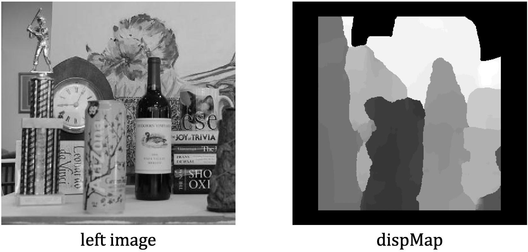
The disparity map contains disparity values that range from -16 (the front-most surface of the Arizona can) to +17 (the back wall). In the above visualization, the front surfaces (closest to the camera) are shown with darker grays and the back surfaces (furthest away from the camera) are shown as white. Along the border of the dispMap matrix, and in two areas at the top of the back wall, there are locations where disparity values were not computed. In the case of the two areas at the top of the back wall, no disparity values were computed because the average contrast in the image was too low to obtain a reliable stereo match. In locations of the dispMap matrix where no disparity is computed, the value -25 is stored (outside the range of valid disparities), which is displayed as black in the visualization above.

Define a function named borders with three inputs and one output:

function ownership = borders (dmap, nodisp, threshold)

dmap is the input disparity map and nodisp is the value that is stored in the disparity map that indicates locations where no valid disparity value was computed (-25 in this example). The input threshold is the size of the change in disparity that will be considered a significant change (a threshold value of 2 works well). This new function should be placed inside your stereo folder.

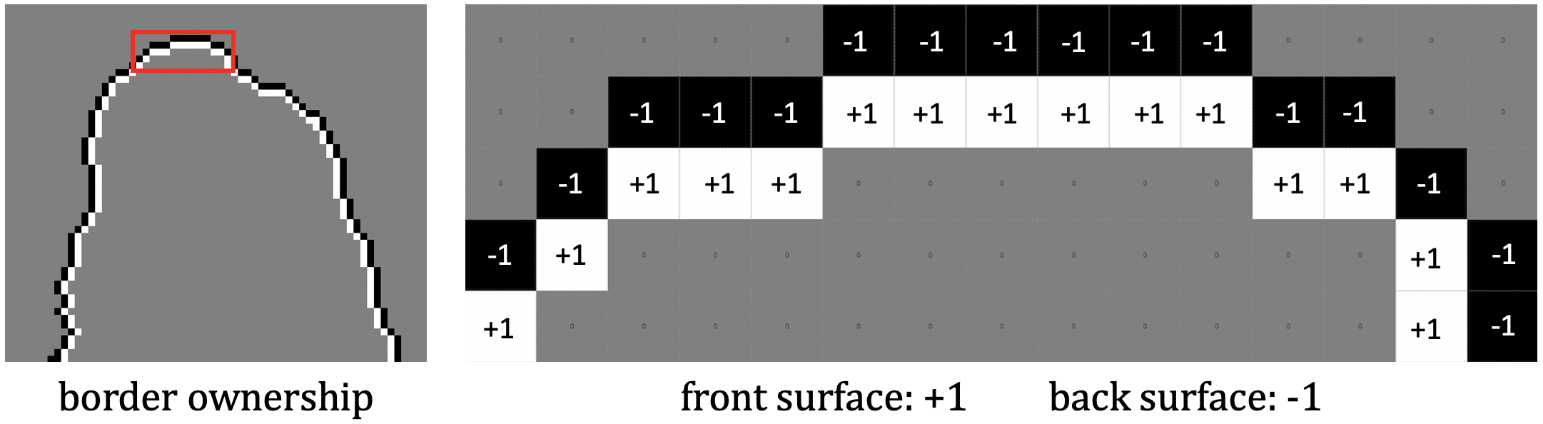
For each location of the input disparity map, the borders function should check whether there is a significant change in disparity (above the input threshold) from its two neighbors to the left or above, and if so, store values in the output ownership matrix that encode the location of the front and back surfaces at this location. The front and back surfaces can be encoded with the values +1 and -1, respectively. The figure below on the left, displays a small region of the result around the top of the wine bottle in the scene. The white pixels indicate locations of the front surface (which "owns" the border), just inside the border, and black pixels indicate locations of the back surface, just outside the border. On the right, the region highlighted with the red rectangle is shown enlarged, with the values of +1 and -1 indicating the front and back surfaces around the border:

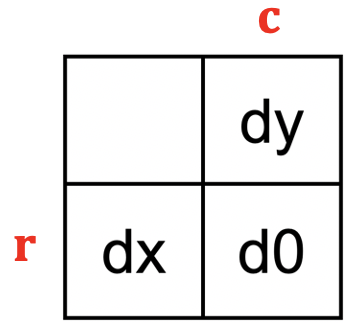
To compute the border ownership encoding, visit each location of the input disparity map. Let r and c denote the row and column of the location currently under consideration. At each location, examine the disparities stored at the current location (r,c) and its neighbors to the left and above, labeled d0, dx, and dy in the diagram below:

First check that none of the three disparity values are the input nodisp value in the function header, which indicates that no disparity was computed at the particular location. If all three locations contain a valid disparity, then examine the pair of values d0 and dx. If there is a significant change in disparity (above the input threshold), then store +1 in the ownership matrix, at the location of the front surface and store -1 at the location of the back surface. Then consider the current location and its neighbor above and apply the same logic.

The following three statements load the disparity map, call the borders function, and display the results:

load dispMap.mat
ownership = borders(dispMap, -25, 2);
imtool(ownership, [-1 1])

Problem 3 (20 points): The Marr-Poggio-Grimson Multi-resolution Stereo Algorithm

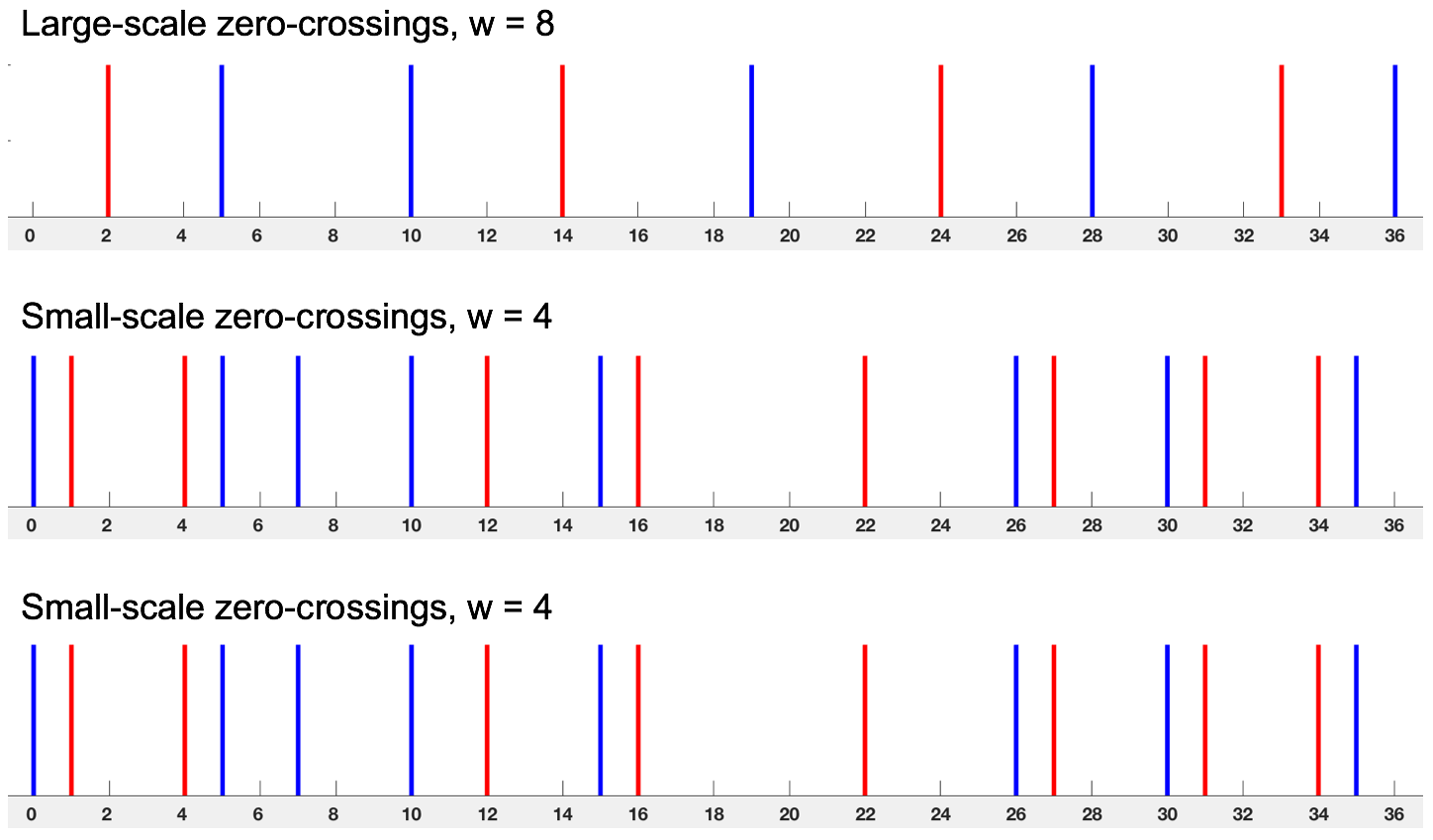
The video on the Marr-Poggio-Grimson Stereo Algorithm describes a simplified version of the MPG multi-resolution stereo algorithm and includes a hand simulation of this algorithm. This problem provides another example for you to hand simulate on your own. The zero-crossing locations are shown in the diagrams below. The top row shows zero-crossing segments obtained from a Laplacian-of-Gaussian operator whose central positive diameter is w = 8, and the bottom two rows show zero-crossing segments obtained from an operator with w = 4. Assume that the matching tolerance m (the search range) is m = w/2. In the diagram, the red lines represent zero-crossings obtained from the left image and the blue lines are zero-crossings from the right image (assume that they are all zero-crossings of the same sign). The axis below the zero-crossings indicates their horizontal position in the image.

Part a: Match the large-scale zero-crossing segments. In your answer, indicate which left-right pairs of zero-crossings are matched and indicate their disparities.

Part b: Match the small-scale zero-crossings, ignoring the previous results from the large-scale matching. In your answer, indicate which left-right pairs of zero-crossings are matched and indicate their disparities. Show your analysis for this case on the bottom row of the figure.

Part c: Match the small-scale zero-crossings again. This time exploit the previous results from the large-scale matching. Show your analysis for this case on the middle row of the figure.

Part d: What are the final disparities computed by the algorithm, based on the matches from Part c? The final disparity is defined as the shift in position between the original location of the left zero-crossings and the location of their matching right zero-crossings.

Part e: One of the constraints that is used in all algorithms for solving the stereo correspondence problem is the continuity constraint. What is the continuity constraint, and how is it incorporated in the simple version of the MPG stereo algorithm that you hand-simulated in this problem?

 

Problem 4 (10 points): Multi-resolution Region-Based Stereo Algorithm

Using the ideas that were embodied in the multi-resolution stereo algorithm developed by Marr, Poggio, and Grimson, describe how the region-based stereo algorithm explored in Problem 2 could be modified to use multiple spatial scales. You can either consider the ideas embodied in the original multi-resolution stereo algorithm proposed to account for the use of multiple spatial scales and eye movements in human stereo processing, or the simplified version of the algorithm that you hand-simulated in Problem 3. You do not need to implement anything here, just describe a possible strategy in words.