Assignment 5
![]()
|
|
Computation for the Sciences
Assignment 5
|
|
Your hardcopy submission should include printouts of all code files that you wrote to solve the two problems below.
assign5_programs folder from the download directory onto your
Desktop. Rename the folder to be yours, e.g.
stella_assign5_programs. Set the MATLAB's Current Directory
appropriately. The
assign5_programs folder contains only one
function, transformView (needed for Problem 1). You will write
all the rest of the MATLAB code from scratch for this assignment. It also contains two
data files, named mathworks.mat and widget.xls to be used in Problem 2.
When you are done with this assignment, you should have all the
code files stored in your assign5_programs folder that you
wrote in addition to the files that we supplied for you.
For this problem, you will work with a set of images from a healthy patient. Single MRI images are called slices. The images below are 27 horizontal slices (click on image to enlarge):

| Brain slices can be viewed on these three planes: horizontal (yellow), sagittal (blue) and coronal (pink) (see Figure at right). Although the slices above are horizontal (sometimes also referred to as axial) slices, we can use MATLAB to figure out how to display sagittal and coronal views of the same brain. |

|
Your goal for this problem is to write an interactive MATLAB program that allows the user to view the MRI data above in different ways.
There is a MATLAB file called mri.mat available online here:
mri.mat.
You can use urlwrite to save the contents of the URL to a local file, then use
load to load mri.mat into MATLAB.
(Check the online MATLAB documentation
for the urlwrite command.)
Load the file mri.mat. Variables D containing the MRI slices, and
a colormap map are created in your workspace. The
matrix D is 128 x 128 x 1 x 27. Each of the 27
horizontal slices is 128 pixels wide by 128 pixels high. The first
dimension runs from the front to the back of the head; the second
dimension runs from left to right; the third dimension contains color
information; and the fourth dimension runs from the bottom (1st slice)
to the top of the head (27th slice).
By manipulating the matrix D,
different slices of the brain can be selected and viewed by your
program.
You will write an interactive program called mri.m that
allows the user to choose from several options (some options may need
to ask the user for more input, for example, which slice to view).
Specifically, your program must perform these tasks:
 >> mri
    Welcome to my program!
    Enter 1 to show all images at once
          2 to display a horizontal slice
          3 to show all frames as a movie
          4 to display a sagittal slice
          5 to display a coronal slice
          e to exit
   ==> 1
     Enter 1(all), 2(horiz.), 3(movie), 4(sag.), 5(cor.) or [e]xit
   ==> 2
    Select a horizontal slice bottom->top [1-27]: 15

     Enter 1(all), 2(horiz.), 3(movie), 4(sag.), 5(cor.) or [e]xit
   ==> 3
     Enter 1(all), 2(horiz.), 3(movie), 4(sag.), 5(cor.) or [e]xit
   ==> 4
     Select a sagittal slice left->right [1-128]: 80

     Enter 1(all), 2(horiz.), 3(movie), 4(sag.), 5(cor.) or [e]xit
   ==> 5
     Select a coronal slice front->back [1-128]: 75
   ==> e
>>
>>
| Option 1 montage |
Option 2 horiz. slice 15 |
Option 3 movie |
Option 4 sagittal slice 80 |
Option 5 coronal slice 75 |

|

|

|

|

|
Programming Notes/Hints:
mri in the mri.m file, and write separate functions to implement each of the 5 tasks listed above (some of these functions may be very short).
mri function cannot directly access data in global workspace, so you need to load mri inside the mri function to store the variables D and map in the local workspace.
montage.
hot (a built-in MATLAB colormap -- doc colormap to learn more). You can choose to use a single colormap, multiple colormaps,
or use none at all in your displays of the MRI slices for this
program. imshow can be called with an optional second input that is the name of a colormap. For example, imshow(rice, hot) uses the hot colormap to display the rice image.
immovie
to create the movie and movie to play the movie.
squeeze and transformView.
squeeze removes singleton dimensions
from a matrix. For example, squeeze(rand(4,1,2)) is 4-by-2.
Selecting one slice from the matrix D in a different plane creates
singleton dimensions that you can discard with squeeze.
transformView that will transform a slice
from one view to another. You do not need to make any changes to this function. Here is an example of how to use
transformView: % the slice variable contains a sagittal view % transforms sagittal view for optimal display newslice = transformView(slice);Now you can show the
newslice in a figure, as usual.
The same transformView function will work for converting horizontal
into coronal views as well.
mri.m.
You should include detailed comments within each file or function that you
submit. You can copy-and-paste together your hardcopy solutions to save paper (rather than printing each function on a separate piece of paper).
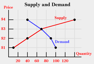
A competitive market has many buyers and sellers of the same goods or services, and is described well by the supply and demand model. In this model, the quantity of a good supplied by a producer and the quantity demanded by the consumer both depend on the price of the good. The law of supply says that the higher the price, the more the producer will supply, while the law of demand says that the higher the price, the less the consumer will demand. The diagram below shows simple supply and demand curves that capture these relationships between the price of a good and the quantity that is supplied by the producer or demanded by the consumer. The law of supply and demand says that the market price of the product will settle at the intersection of the supply and demand curves, called the equilibrium point. If the price is too low, then consumers will demand more than the producer is willing to supply, leading to a shortage of the good and willingness of consumers to pay more, driving the price up. On the other hand, if the price is too high, producers may produce more than consumers will buy, leading producers to lower the price. At the equilibrium point, the price of the product is set so that producers sell exactly the same quantity of goods that consumers will buy.
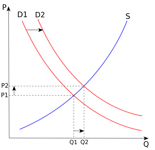
Changes in the overall demand for, or supply of a product can shift the equilibrium point. In the picture below, demand increases from the curve D1 to the curve D2, while the supply curve remains the same. This leads to an increase in the equilibrium price, from P1 to P2.
In this problem, you will write a program that allows the user to explore the interaction between supply and demand for two small markets. The first is the market for a new student version of MATLAB supplied by Mathworks, Inc., and the second is the market for a new widget supplied by J. J. Widget Co. This problem will also give you practice with creating a larger program that integrates multiple code files that implement different aspects of the task. There are four subtasks in this case: (1) loading the data for the supply and demand curves, (2) computing the equilibrium point, (3) displaying the results and (4) controlling the overall process. Parts (1)-(3) can be written and tested independently. The next four sections describe each of the four parts of the program.
Write a function that loads in the supply and demand data from a file and returns the
data in four output vectors that store the prices and quantities for the supply and
demand curves. There are two sources of data for this problem. For the first source, imagine
that Mathworks, Inc. is planning to launch a new student version of MATLAB and conducts a market
survey to determine a reasonable price for this new product. The survey data, shown below,
indicates the expected quantities of MATLAB that students will demand at a set of prices shown
in the first column, for six broad areas of the US. The numerical data in the table is stored
in a variable matlabDemand in the file mathworks.mat in the
assign7_programs folder.
        area1   area2   area3   area4   area5   area6
$175     500     540     460     525     575     475
$150     600     650     550     620     660     580
$125     800     845     740     820     880     760
$100    1100    1160    1050    1130    1170    1070
$75     1500    1550    1445    1525    1585    1480
$50     2000    2055    1955    2030    2080    1985
For this data, the total quantity that students will purchase at each price is
the sum of the quantities for the six areas. The variable matlabSupply in the
mathworks.mat file stores the data in the following table, which
indicates the quantity that Mathworks, Inc. is willing to supply for each of
the same prices:
       quantity
$175     7250
$150     6750
$125     6000
$100     5000
$75      3500
$50      1000
Write a function that computes and returns the equilibrium price and quantity, given six inputs: the prices and quantities for the supply and demand curves, and optional changes in supply or demand. Consider developing this function in two steps, where the first step determines the equilibrium point without allowing a change in supply or demand. One strategy for finding the intersection of the supply and demand curves is to fit each set of data with a smooth curve such as a quadratic function, and then determine where these two functions cross each other. Suppose you want to approximate the supply and demand curves with a quadratic function of the form:
y = ax2 + bx + c
where x represents quantity and y represents price. The function polyfit calculates
the coefficients of a polynomial function of degree n that best fits a given set of points, and
returns a vector of these coefficients. This function has three inputs corresponding to the
x and y coordinates of the points and the degree of the polynomial.
The companion function polyval calculates the values of a polynomial
function given a vector of its coefficients and a vector of x
values. In the following example, a set of x and y values
are first generated from a known polynomial with coefficients 2, 3 and -10. polyfit
is then used to derive these coefficients from the x and y values, and the coefficients are
used to calculate values of this polynomial for a different set of x coordinates.
>>
>> x = -5:5
   -5   -4   -3   -2   -1    0    1    2    3    4    5
>> y = 2*x.^2 + 3*x - 10
   25   10   -1   -8  -11  -10   -5    4   17   34   55
>> coeffs = polyfit(x, y, 2)
   2.0000  3.0000  -10.0000
>> x2 = 4:10
    4    5    6    7    8    9   10
>> y2 = polyval(coeffs, x2)
  34.0000  55.0000  80.0000  109.0000  142.0000  179.0000  220.0000
>>
You can use polyfit to compute the coefficients of quadratic functions that
approximate the supply and demand curves, and use polyval to construct a set of
at least 100 samples of each of these curves over the range of quantities spanned by the
data. The samples of the two curves can then be used to estimate the price and quantity of the
equilibrium point. Hints: At the intersection point, the absolute
value of the difference between the two curves reaches a minimum, and recall that
the min function can return a second output that is the index of the minimum
value of a function.
At the end of your function that computes the equilibrium point, call your display function (described in the next section) to display the supply and demand curves and the computed equilibrium point. Note that the computed intersection may be shifted slightly from the apparent intersection, due to the quadratic approximation of the curves.
After you complete this first step, then add the ability to change the overall supply or demand, in order to explore its effect. One way to model an increase in supply or demand is to shift the original supply or demand curves to the right, reflecting an increase in the quantities of the product that people are willing to buy at each price, or an increase in the quantities that the company will sell at each price. Analogously, a decrease in supply or demand can be modelled as a shift to the left of the supply or demand curve. There are different ways that the user could specify the amount of increase or decrease to test. In this problem, the quantities of MATLAB and widgets are on very different scales (roughly 3000-12000 vs. 0-60). One way to specify an amount to change supply or demand is to enter a factor to be multiplied by the maximum quantity in the data. For example, the factor 0.1, when multiplied by the maximum MATLAB and widget quantities would yield 1200 and 6, respectively. Thus, specifying a factor of 0.1 for the change in supply or demand would increase the quantities of MATLAB supplied or demanded at each price by 1200, or increase the quantities of widgets by 6. A factor of -0.1 would decrease these quantities by 1200 or 6. Modify your function for computing the equilibrium point so that it has two optional inputs for specifying the factors to use to change supply and demand, and use these factors to adjust the quantities for the supply and demand curves before computing the equilibrium point. These two inputs can have default values of 0.
Write a function that displays the supply and demand curves, and highlights the equilibrium point. A sample display is shown below:

This function will need to have six inputs: the prices and quantities for the supply curve,
the prices and quantities for the demand curve, and the equilibrium price and quantity. A
single dot can be displayed at a location (x,y) using the scatter
function, for example:
>> scatter(x, y, 50, 'k', 'filled')
(see help scatter for more information).
Your display function should give the user the option of keeping the current plots on the
display, or clearing the current display. You can implement and test this function before
completing the function that computes the equilibrium point - just "eyeball" the data and
call this function with approximate coordinates for the equilibrium point.
Finally, write a high-level script that controls the overall flow of the program. This script should print some introductory information to the user about what the program does, call the functions to load the data and compute the equilibrium point, print the resulting equilibrium price and quantity, and then incorporate a loop that allows the user to specify changes in the supply or demand curves and observe the resulting changes in the equilibrium point. The following interaction illustrates one example of how a user might interact with your program - the user's input is shown in bold:
>> supplyDemand
Welcome to the CS112 Supply and Demand program!
Select a data source, view supply and demand curves,
see the equilibrium price and quantity, and explore
how these values change with supply and demand :)
select the data to analyze: mathworks (1) or widget (2): 1
keep current display? yes (1) no (0): 0
Equilibrium price: $116.7817
Equilibrium quantity: $5602.0721
specify the change in supply or demand as a fraction of the
maximum quantity present in the current supply or demand curves
change in supply (-0.5 to 0.5): 0.0
change in demand (-0.5 to 0.5): 0.1
keep current display? yes (1) no (0): 1
Equilibrium price: $130.3746
Equilibrium quantity: $6066.7372
keep going? yes (1), no(0): 1
change in supply (-0.5 to 0.5): 0.0
change in demand (-0.5 to 0.5): -0.1
keep current display? yes (1) no (0): 1
Equilibrium price: $104.4731
Equilibrium quantity: $5140.041
keep going? yes (1), no(0): 0
>>
You are welcome to modify the text as you'd like, and use a different range of factors for specifying changes in supply and demand. The above interaction resulted in the following display:

Be sure to thoroughly test your code. For your hardcopy submission, hand in the four code files that you wrote, which you can cut and paste into a single file.