Reading on Bézier Curves and Surfaces

Please also read this, on using Quadratic and Cubic Bézier curves in the HTML5 Canvas:

HTML Canvas and Bézier curves

Additional Reading

Most of what I know about Curves and Surfaces I learned from Angel's book, so check that chapter first. It's pretty mathematical in places, though. There's also a chapter of the Red Book (the Red OpenGL Programming Guide).

For practical programming in Three.js, you might try this page on rendering lines and Bézier Curves in Three.js and WebGL.

Organization

This reading is organized as follows. First, we look at why we try to represent curves and surfaces in graphics models, but I think most of us are already pretty motivated by that. Then, we look at major classes of mathematical functions, discussing the pros and cons, and finally choosing cubic parametric equations. Next, we describe different ways to specify a cubic equation, and we ultimately settle on Bézier curves. Finally, we look at how the mathematical tools that we've discussed are reflected in OpenGL code.

The preceding develops curves (that is, 1D objects --- wiggly lines). In graphics, we're mostly interested in surfaces (that is, 2D objects --- wiggly planes). The last sections define surfaces as a generalization of what we've already done with curves.

Introduction

Representing Curves

• explicit equations
• implicit equations
• parametric equations

Explicit Equations

The explicit equations are the ones we're most familiar with. For example, consider the following functions: $$ \begin{eqnarray*} y &=& mx+b\\ y &=& ax^2+bx+c\\ y &=& \sqrt{r^2-x^2}\\ \end{eqnarray*} $$

An explicit equation has one variable that is dependent on the others; here it is always $y$ that is the dependent variable: the one that is calculated as a function of the others.

An advantage of the explicit form is that it's pretty easy to compute a bunch of values on the curve: just iterate $x$ from some minimum to some maximum.

One trouble with the explicit form is that there are often special cases (for example, vertical lines). Another is that the limits on $x$ will change from function to function (the domain is infinite for the first two examples, but limited to $\pm r$ for the third). The deadly blow is that it's hard to handle non-functions, such as a complete circle, or a parabola of the form $x=ay^2+by+c$. You could certainly get a computer program to handle this form, but you'd need to encode lots of extra stuff, like which variable is the dependent one and so forth. Bézier curves can be completely specified by just an array of coefficients.

Implicit Equations

Another class of representations are implicit equations. These equations always put everything on one side of the equation, so no variable is distinguished as the dependent one. For example: \begin{eqnarray*} ax+by+cz-d=0 & & \textrm{plane} \\ ax^2+by^2+cz^2-d^2=0 & & \textrm{egg} \\ \end{eqnarray*}

These equations have a nice advantage that, given a point, it's easy to tell whether it's on the curve or not: just evaluate the function and see if the function is zero. Moreover, each of these functions divides space in two: the points where the function is negative and the points where it's positive. Interestingly, the surfaces do as well, so the sign of the function value tells you which side of the surface you're on. (It can even tell you how close you are.)

The fact that no variable is distinguished helps to handle special cases. In fact, it would be pretty easy to define a large general polynomial in $x$, $y$ and $z$ as our representation.

The deadly blow for this representation, though, is that it's hard to generate points on the surface. Imagine that I give you a value for $a$, $b$, $c$ and $d$ and you have to find a value for $x$, $y$, and $z$ that work for the two examples above. Not easy in general. Also, it's hard to do curves (wiggly lines). In general, curves are the intersection of two surfaces, like conic sections (parabola, ellipse, etc.) being the intersection of a cone and a plane

Parametric Equations

Finally, we turn to the parametric equations. We've seen these before, of course, in defining lines, which are just straight curves.

With parametric equations, we invent some new variables,parameters, typically $s$ and $t$. These variables are then used to define a function for each coordinate: \[ \vecIII{x(s,t)}{y(s,t)}{z(s,t)} \]

Parametric functions have the advantage that they're easy to generalize to 3D, as we already saw with lines.

The parameters tell us where we are on the surface (or curve) rather than where we are in space. Therefore, we have a conventional domain, namely the unit interval. That means that, like our line segments, our curves will all go from $t=0$ to $t=1$. (They don't have to, but they almost always do.) Similarly, surfaces are all points where $0\leq s,t \leq 1$. Thus, another advantage of parametric equations is that it's easy to define finite segments and sheets, by limiting the domains of the parameters.

The problem that remains is what family of functions we will use for the parametric functions. One standard approach is to use polynomials, thereby avoiding trigonometric and exponential functions, which are expensive to compute. In fact, we usually choose a cubic:

Another problem comes with finding these coefficients. We'll develop that in later sections, but the solution is essentially to appeal to some nice techniques from linear algebra that let us solve for the desired coefficients given some desired constraints on the curve, such as where it starts and where it stops.

Why We Want Low Degree

Why do we typically use a cubic? Why not something of higher degree, which would let us have more wiggles in our curves and surfaces? This is a reasonable question.

In general, we want a low degree: quadratic, cubic or something in that neighborhood. There are several reasons:

1. The resulting curve is smooth and predictable over long spans. In other words, because it wiggles less, we can control it more easily. Consider trying to make a nice smooth curve with a piece of cardboard or thin wood (a literal spline) versus with a piece of string.
2. It takes less information to specify the curve. Since there are four unknown coefficients, we need four points (or similar constraints) to solve for the coefficients. If we were using a quartic, we'd need 5 points, and so forth.
3. If we want more wiggles, we can join up several splines. Because of the low degree, we have good control of the derivative at the end points, so we can make sure that the curve is smooth through the joint.
4. Finally, it's just less computation and therefore easier for the graphics card to render.

OpenGL will permit you to use higher (and lower) degree functions, but for this presentation we'll stick to cubics. If you'd like to play with higher degree functions, I'm happy to help you with that. The following figure shows four points defining a curve.

Joining Curves

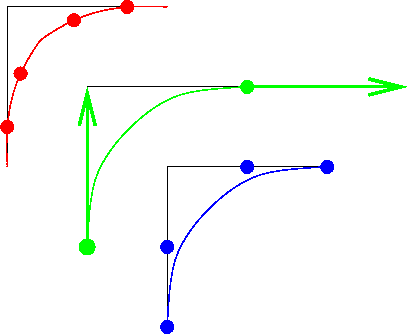
To make longer curves with more wiggles, we can join up several Bézier curves. The following figure shows two examples. In the first, the curves are connected (the last control point of the first curve is the same as the first point of the second), but not smooth through the joint. The second manages to make the joint smooth, by making sure the tangents line up. The tangents are defined by the line segments from P2 to P3 and from Q0 to Q1. So, if P2, P3=Q0, and Q1 are co-linear, the joint will be smooth. (We'll revisit this later.)

Ways of Specifying a Curve

Once we've settle on a family of functions, such as cubics, what remains is determining the values of the coefficients that give us a particular curve. To define a cubic, we need four pieces of information, though there are different choices about what four pieces of information. If I want, for example, a curve that looks like the letter ``J,'' what four pieces of information do I have to specify? It turns out that there are three major ways of doing that. (It's strange how everying seems to break down into threes in this subject.)

• Interpolation: That is, you specify four points on the curve and the curve goes through (interpolates) the points. This is pretty intuitive, and a lot of drawing programs allow you to do this, but it's not often used in CG. This is primarily because such curves have an annoying way of suddenly lurching as they struggle to get through the next specified point.

  One exception is that this technique is often used when you have a lot of data, as with a digitally scanned face or figure. Then you have thousands of points, and the curve pretty much has no choice but to be what you want (although the graphics artist may still want to do some smoothing, say for measurement error or something).

• Hermite: In the Hermite case, the four pieces of information you specify are 2 points and 2 vectors: the points are where the curve starts and ends, and the vectors indicate the direction of the curve at that point. They are, in fact, derivatives. (If you've done single-dimensional calculus, you know that the derivative gives the slope at any point and the slope is just the direction of the line; the same idea holds in more dimensions.) This is a very important technique, because we often have this information. For example, if I want a nice rounded corner on a square box, I know the slope at the beginning (vertical, say) and at the end (horizontal).
• Bézier: With a Bézier curve, we specify 4 points, as follows: the curve starts at one, heading for second, ends at fourth, coming from third. (See the picture below.) This is a very important technique, because you can easily specify a point using a GUI, while a vector is a little harder. It turns out there are other reasons that Bézier is preferred, and in practice the first two techniques are implemented by finding the Bézier points that draw the desired curve.

The figure above compares these three approaches. An X11 drawing program that will let you experiment with the examples drawn in the figure is xfig. (Xfig uses quadratic Bézier curves.) Try it! You can also draw Bézier curves in the HTML5 2D canvas.

OpenGL curves are drawn by calculating points on the line and drawing straight line segments between those points. The more segments, the smoother the resulting curve looks. In some implementations, the calculations can be done by the graphics card. In THREE.js, they compute the vertices in the main processor, rather than having the graphics card do that. I believe it's because they want to simplify the shader program, but that's a guess.

Solving for the Coefficients

We'll now discuss how we can solve for the coefficients given the control information (the four points or the two points and two vectors). Essentially, we're solving four simultaneous equations. We won't do all the gory details, but we'll appeal to some results from linear algebra.

Let's look at how we solve for the coefficients in the case of the interpolation curves; the others work similarly.

Note that in every case, the parameter is $t$ and it goes from 0 to 1. For the interpolation curve, the interior points are at $t=1/3$ and $t=2/3$. Let's focus just on the function for $x(t)$. The other dimensions work the same way. If we substitute $t=\{0, \frac13, \frac23, 1 \}$ into the cubic equations we saw earlier, we get the following: \begin{eqnarray*} && P_0 = x(0) = C_0\\ && P_1 = x(1/3) = C_0+\frac13C_1 + \left(\frac13\right)^2C_2 + \left(\frac13\right)^3C_3\\ && P_2 = x(2/3) = C_0+\frac23C_1 + \left(\frac23\right)^2C_2 + \left(\frac23\right)^3C_3\\ && P_3 = x(1) = C_0+C_1 + C_2 + C_3\\ \end{eqnarray*}

What does this mean? It means that the $x$ coordinate of the first point, $P_0$, is $x(0)$ This makes sense: since the function $x$ starts at $P_0$, it should evaluate to $P_0$ at $t=0$. (This is also exactly what happens with a parametric equation for a straight line: at $t=0$, the function evaluates to the first point.) Similarly, the $x$ coordinate of the second point, $P_1$ is $x(1/3)$ and that evaluates to the expression that you see there. Most of those coefficients are still unknown, but we'll get to how to find them soon enough.

Putting these four equations into a matrix notation, we get the following: \[ \mathbf{P} = \left[ \begin{array}{cccc} 1 & 0 & 0 & 0 \\ 1 & \frac13 & (\frac13)^2 & (\frac13)^3 \\ 1 & \frac23 & (\frac23)^2 & (\frac23)^3 \\ 1 & 1 & 1 & 1 \\ \end{array}\right] \mathbf{C} \]

The $\mathbf{P}$ matrix is a matrix of points. It could just be the $x$ coordinates of our points $P$, or more generally it could be a matrix each of whose four entries is an $(x,y,z)$ point. We'll view it as a matrix of points. The matrix $\mathbf{C}$ is a matrix of coefficients, where each element --- each coefficient --- is a triple $(C_x,C_y,C_z)$, meaning the coefficients of the $x(t)$ function, the $y(t)$ function and the $z(t)$ function.

If we let $\mathbf{A}$ stand for the array of numbers, we get the following deceptively simple equation: \[ \mathbf{P} = \mathbf{A} \mathbf{C} \]

By inverting the matrix $\mathbf{A}$, we can solve for the coefficients! (The inverse of a matrix is the analog to a reciprocal in scalar mathematics. It's also equivalent to solving the simultaneous equations in a very general way.) The inverse of $\mathbf{A}$ is called the interpolating geometry matrix and is denoted $\mathbf{M}_I$: \[ \mathbf{M}_I = \mathbf{A}^{-1} \]

Notice that the matrix $\mathbf{M}_I$ does not depend on the particular points we choose, so that matrix can simply be stored in the graphics card. When we send an array of control points, $\mathbf{P}$, down the pipeline, the graphics card can easily compute the coefficients it needs for calculating points on the curve: \[ \mathbf{C} = \mathbf{M}_I \mathbf{P} \]

The same approach works with Hermite and Bézier curves, yielding the Hermite geometry matrix and the Bézier geometry matrix. In the Hermite case, we take the derivative of the cubic and evaluate it at the endpoints and set it equal to our desired vector (instead of points $P_1$ and $P_2$). In the Bézier case, we use a point to define the vector and reduce it to the previously solved Hermite case.

Blending Functions

Sometimes, looking at the function in a different way can give us additional insight. Instead of looking at the functions in terms of control points and geometry matrices, let's look at them in terms of how the control points influence the curve points.

Looking just at the functions of $t$ that are combined with the control points, we can get a sense of the influence each control point has over each curve point. The influences of the control points are blended to yield the final curve point, and these functions are called blending functions. (Blending functions are also important for understanding NURBS, a generalization of Bézier curves.) Equivalently, the curve points are a weighted average of the control points, where the blending functions give the weight. (We looked at weighted averages in our discussion of bi-linear interpolation.) That is, if you evaluate the four blending functions at a particular parameter value, $t$, you get four numbers, and those numbers are weights in a weighted sum of the four control points.

The following function gives the curve, $P(t)$, as a weighted sum of the four control points, where the four blending functions evaluate to the appropriate weight as a function of $t$. \begin{eqnarray*} P(t) &=& B_0(t)*P_0 + B_1(t)*P_1 + B_2(t)*P_2 + B_3(t)*P_3 \end{eqnarray*}

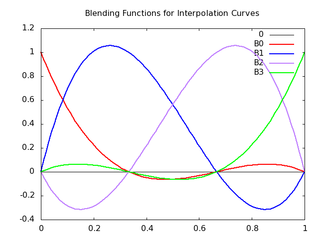
The following are the blending functions for interpolating curves. \begin{eqnarray*} B_0(t) &=& \frac{-9}2(t-\frac13)(t-\frac23)(t-1) \\ B_1(t) &=& \frac{27}2t(t-\frac23)(t-1) \\ B_2(t) &=& \frac{-27}2t(t-\frac13)(t-1) \\ B_3(t) &=& \frac{-9}2t(t-\frac13)(t-\frac23) \\ \end{eqnarray*}

These functions are plotted in the following figure on blending functions for Interpolation Curves.

Alternatively, you can go over to Wolfram Alpha and see the live plotting (and adjust to your taste) by clicking on these links

plot (-9/2)(t-(1/3))(t-(2/3))(t-1) from t=0 to 1

plot (-9/2)(t-(1/3))(t-(2/3))(t-1), (27/2)t(t-(2/3))(t-1), (-27/2)t(t-(1/3))(t-1) from t=0 to 1

plot (-9/2)(t-(1/3))(t-(2/3))(t-1), (27/2)t(t-(2/3))(t-1), (-27/2)t(t-(1/3))(t-1), (-9/2)t(t-(1/3))(t-(2/3)) from t=0 to 1

plot (-9/2)(t-(1/3))(t-(2/3))(t-1), (27/2)t(t-(2/3))(t-1), (-27/2)t(t-(1/3))(t-1), (-9/2)t(t-(1/3))(t-(2/3)) from t=0 to 1

First, notice that the curves always sum to 1. (It may not be entirely obvious, but it's true.) When a curve is near zero, the control point has little influence. When a curve is high, the weight is high and the associated control point has a lot of influence: a lot of pull. In fact, when a control point has a lot of pull, the curve passes near it. When a weight is 1, the curve goes through the control point.

Notice that the blending functions are negative sometimes (they all start and end at zero), which means that this isn't a normal weighted average. (A normal weighted average has all non-negative weights.) What would a negative weight mean? If a positive weight means that a control point has a certain pull, a negative value gives it push --- the curve is repelled from that control point. This repulsion effect is part of the reason that interpolation curves are hard to control.

Hermite Representation

The coefficients for the Hermite curves and therefore the blending functions can be computed from the control points in a similar way (we have to deal with derivatives, but that's not the point right now).

Note that the derivative (tangent) of a curve in 3D is a 3D vector, indicating the direction of the curve at this moment. (This follows directly from the fact that if you subtract two points, you get the vector between them. The derivative of a curve is simply the limit as the points you're subtracting become infinitely close to each other.)

The Hermite blending functions are the following. \[ \mathbf{b}(t) = \vecIV {2t^3-3t^2+1} {-2t^3+3t^2} {t^3-2t^2+t} {t^3-t^2} \]

The Hermite blending functions are plotted in the following figure:

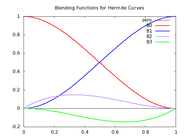
The Hermite curves have several advantages:

• Smoothness:
  • easier to join up at endpoints. Because we control the derivative (direction) of the curve at the endpoints, we can ensure that when we join up two Hermite curves that the curve is smooth through the joint: just ensure that the second curve starts with the same derivative that the first one ends with.
  • The blending functions don't have zeros in the interval: so the influence of a control point never switches from positive to negative. For example, the influence of the first control point peaks at the beginning and steadily, monotonically, drops to zero over the interval.
• The Hermite can be easier to control. As we mentioned earlier, there's no need to know interior points, and we often only know how we want a curve to start and end.

Bézier Curves

The Bézier curve is based on the Hermite, but instead of using vectors, we use two control points. Those control points are not interpolated though: they exist only in order to define the vectors for the Hermite, as follows: \begin{eqnarray*} p'(0) &=& \frac{p_1-p_0}{1/3} = 3(p_1-p_0)\\ p'(1) &=& \frac{p_3-p_2}{1/3} = 3(p_3-p_2) \end{eqnarray*}

That is, the derivative vector at the beginning is just three times the vector from the first control point to the second, and similarly for the other vector. The figure below shows the derivative vectors and the Bézier control points. Notice (as we can see from the equations above), that the vectors are three times longer than the distance of the inner control points from the end control points. However, that's not important. The factor is chosen so that the resulting equations are simplified.

Like the Hermite, Bézier curves are easily joined up. We can easily get continuity through a joint by making sure that the last two control points of the first curve line up with the first two control points of the next. Even better, the interior control points should be equally distant from the joint. This ensures that the derivatives are equal and not just proportional. You can see this in the earlier figure where we smoothly joined two Bézier curves. Repeating that figure here:

• The last control point of the green curve (P3) is the same as the first point of the red curve (Q0).
• The three points (P2, P3=Q0, Q1) form a straight line. (In this case it's a vertical line, but that was just for my convenience.) That co-linearity means that the derivatives are in the same direction, so the joint is smooth.
• The distance from P2-P3 is the same as the distance from Q0-Q1, so that the derivatives are not just lined up but are actually equal. This gives extra smoothness.

The Bézier blending functions are especially nice, as seen in following equation.

Here is a figure that plots the Bézier blending functions:

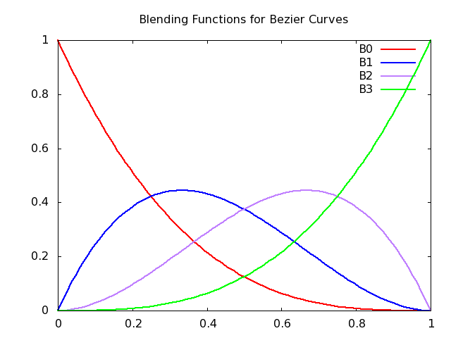
These blending functions are from a family of functions called the Bernstein polynomials: \[ b_{kd}(t) = \Choose{d}{k} t^k(1-t)^{d-k} \]

These can be shown to:

• Have all roots at 0 and 1
• Be non-negative in the interval [0,1]
• Be bounded by 1
• Sum to 1

Perfect for mixing! Thus, our Bézier curve is a weighted sum, so geometrically, all points must lie within the convex hull of the control points, as shown in the following figure:

To be concrete, let's take an example of the Bézier blending functions. For example, what is the midpoint of a Bézier curve? The midpoint is at a parameter value of $u=0.5$. Evaluating the four functions in the Bézier blending functions, we get:

Thus, to find the coordinates of the midpoint of a Bézier curve, we only need to compute this weighted combination of the control points. Essentially: \begin{eqnarray*} P(0.5) &=& \frac18 P_0 + \frac38 P_1 + \frac38 P_2 + \frac18 P_3 \\ &=& (P_0 + 3 P_1 + 3 P_2 + P_3 )/8 \end{eqnarray*}

It turns out that there's a very nice recursive algorithm for computing every point on the curve by successively dividing it in half like this, stopping the recursion when the piece is sufficiently short or flat, so that it can be drawn with just a straight line.

Representing Surface Patches

Using parametric representation, each coordinate becomes a function of two new parameters, which we will call $s$ and $t$, just like we did with textures (which is why $u$ and $v$ are sometimes used instead). \[ \begin{array}{rcllll} x(s,t) &=& C_{00} + &C_{01}t + &C_{02}t^2 + &C_{03}t^3 + \\ & & C_{10}s + &C_{11}st + &C_{12}st^2 + &C_{13}st^3 + \\ & & C_{20}s^2 + &C_{21}s^2t + &C_{12}s^2t^2 + &C_{23}s^2t^3 + \\ & & C_{30}s^3 + &C_{31}s^3t + &C_{22}s^2t^2 + &C_{33}s^3t^3\\ \end{array} \]

or \[ x(s,t) = \sum_{i=0}^{3}\sum_{j=0}^{3} C_{ij}s^it^j \]

And similarly for $y$ and $z$. Since there are 16 coefficients, we need 16 control points to specify the surface patch.

Note that the four edges of a Bézier surface are Bézier curves, which helps a great deal in understanding how to control them. That helps us to understand 12 of the 16 control points.

The four interior points are hard to interpret. Concentrating on one corner: if it lies in the plane determined by the three boundary points, the patch is locally flat. Otherwise, it tends to twist. This is hard to picture. It is, of course, related to the double partial derivative of the curve: \begin{equation} \label{eq:dudv} \frac{\partial^2 p}{\partial u\partial v}(0,0) = 9(p_{00} - p_{01} + p_{10} - p_{11}) \end{equation}

Bézier Patch Demo in THREE.js

The following uses some things that I added to THREE.js, just to automate the computing of the interpolated points and faces.

Dome Surface

You can stop here; the rest is based on the old OpenGL API, rather than Three.js. In the old OpenGL API, you could coax the graphics card into computing the points on curves and surfaces for you, but the more recent approach is to do all that computation in the main CPU and send the computed vertices down to the graphics card. Three.js does this for us when we construct curved geometrical objects.

Bézier Curves in OpenGL

Note for 2014: The following section will have to be theoretical for now, because it seems that the current version of Three.js does not expose the OpenGL Bézier curve API or even use it. Instead, it provides functions for computing values using the Bernstein polynomials, which we can then use for computing vertices for a line or a surface. Please read this for the concepts, but you need not pay close attention to the programming aspects.

To draw a curve in OpenGL, the main thing we have to do is to specify the control points. However, there are other things we might want OpenGL to calculate for us. Here are some:

• vertices (points on the curve or surface)
• normals
• colors
• texture coordinates

They all work the same way. For example, if we specify four control points, we can have OpenGL compute any point on the curve, and if we specify four colors (one for each of those points), we can have OpenGL compute the color of the associated point, using the same blending functions.

Each of these is called an evaluator. You can have multiple evaluators active at once, say for vertices and colors.

The basic OpenGL functions for curves are (in C):

glMap1f(target, u_min, u_max, stride, order, point_array);
glEnable(target);
glEvalCoord1f(u);

The first two are setup functions. The first, glMap1f(), is how we specify all the control information (points, colors, or whatever). The target is the kind of control information you are specifying and the kind of information you want generated, such as:

• GL_MAP1_VERTEX_3, a vertex in 3D
• GL_MAP1_VERTEX_4, a vertex in 4D (homogeneous coordinates
• GL_MAP1_COLOR_4, a RGBA color
• GL_MAP1_NORMAL, a normal vector
• GL_MAP1_TEXTURE_COORD_1, a texture coordinate. (We'll talk about textures in a few weeks.)

The u_min and u_max arguments are just the min and max paramater, so they are typically 0 and 1, though if you just want a piece out of the curve, you can use different values. For example, to get the middle fifth of the curve, you could give u_min=0.4 and u_max=0.6.

The stride is a complicated thing that we'll talk about below. The order is one more than the degree of the polynomial (4 for a cubic) and is therefore equal to the number of control points we are supplying. Since JavaScript knows how long its arrays are, it can count that for you. Finally, an array of the control information: vertices, RGBA values or whatever. They should be of the same type as the target.

The second function, glEnable(), simply enables the evaluator; you can enable and disable them like lights or textures.

Finally, the last function, glEvalCoord1f(), replaces functions like \texttt{glVertexf()}, \texttt{glColorf()} and \texttt{glNormalf()}, depending on the target. In other words, that's the one that actually calculates a point on the curve or its color or whatever, and sends it down the pipeline. Here's an example of how you might do 100 evenly spaced steps on a curve:

glBegin(GL_LINE_STRIP)
for(i = 0; i < 101; i++ ) {
    glEvalCoord1f(i/100.0)    # instead of glVertex3f
}

If you know that you just want evenly spaced steps (which is often the case), you can use the following two functions instead of calls to glEvalCoord.

  glMapGrid1f(steps,u_min,u_max)
  glEvalMesh1(GL_LINE,start,stop)

This is a grid of `steps' (say 100), from the minimum $u$ to the maximum $u$ (typically 0.0 to 1.0, but not necessarily). The second actually evals the mesh from `start' (typically 0) to `stop' (typically the same as `steps').

Strides

What the heck is a stride? Since the control point data is given to OpenGL in one flat array, the stride is the number of elements to skip to get from one row/column to the next row/column.

We saw strides in the context of two-dimensional arrays used to represent color images. The stride from one texel to the next along a row was 3 bytes. The stride from one texel to the next down a column was 3*width, where width is the width of the texture (which is the same as the length of a row, which is the same as the number of columns).

For curves, the stride is almost always 3, because the elements are 3-place coordinates consecutive in memory. If you're specifying colors, the stride will be 4, because the elements are 4-place RGBA values consecutive in memory. The stride becomes more complicated when we deal with 2D surfaces instead of 1D curves.

Representing Surface Patches

Using parametric representation, each coordinate becomes a function of two new parameters, which we will call $s$ and $t$, just like we did with textures (which is why $u$ and $v$ are sometimes used instead). \[ \begin{array}{rcllll} x(s,t) &=& C_{00} + &C_{01}t + &C_{02}t^2 + &C_{03}t^3 + \\ & & C_{10}s + &C_{11}st + &C_{12}st^2 + &C_{13}st^3 + \\ & & C_{20}s^2 + &C_{21}s^2t + &C_{12}s^2t^2 + &C_{23}s^2t^3 + \\ & & C_{30}s^3 + &C_{31}s^3t + &C_{22}s^2t^2 + &C_{33}s^3t^3\\ \end{array} \]

or \[ x(s,t) = \sum_{i=0}^{3}\sum_{j=0}^{3} C_{ij}s^it^j \]

And similarly for $y$ and $z$. Since there are 16 coefficients, we need 16 control points to specify the surface patch.

Note that the four edges of a Bézier surface are Bézier curves, which helps a great deal in understanding how to control them. That helps us to understand 12 of the 16 control points.

The four interior points are hard to interpret. Concentrating on one corner: if it lies in the plane determined by the three boundary points, the patch is locally flat. Otherwise, it tends to twist. This is hard to picture. It is, of course, related to the double partial derivative of the curve: \begin{equation} \label{eq:dudv} \frac{\partial^2 p}{\partial u\partial v}(0,0) = 9(p_{00} - p_{01} + p_{10} - p_{11}) \end{equation}

Bézier Surfaces in OpenGL

Note for 2014: As above, the following section will have to be theoretical for now.

To handle surfaces, we just convert the OpenGL functions from the earlier section above to 2D. The basic functions are:

glMap2f(type, u_min, u_max, u_stride, u_order,
              v_min, v_max, v_stride, v_order, point_array);
glEnable(type);
glEvalCoord2f(u,v);

Here, it's even more common to let OpenGL do the work of generating all the points:

  glMapGrid2f(u_steps,u_min,u_max,v_steps,v_min,v_max)
  glEvalMesh2(GL_FILL,u_start,u_stop,v_start,v_stop)

Texture Mapping

If you're doing texture mapping, you can have OpenGL calculate texture coordinates for you at each of the surface points, just by setting up and enabling that target:

glMap2f(GL_MAP2_TEXTURE_COORD_2, u_min, u_max, v_min, v_max,
        texture_control_point_array)
glEnable(GL_MAP2_TEXTURE_COORD_2)

Because texture-mapping is 2D, the texture coordinates are often generated by a linear Bézier function, such as:

glMap2f(GL_MAP2_TEXTURE_COORD_2, 0, 1, 0, 1,
        [[[0,0], [0,1]],
         [[1,0], [1,1]]]);
glEnable(GL_MAP2_TEXTURE_COORD_2);

Here the texture coordinates (0,0) will correspond to the first spatial corner, and the $(s,t)$ texture coordinates will equal the $(u,v)$ Bézier parameters.

Normal Vectors

If you want to use lighting on a surface, you have to generate normals as well. You can do it yourself using

glMap2f(GL_MAP2_VERTEX_3, u_min, u_max, v_min, v_max, point_array)
glEnable(GL_MAP2_VERTEX_3)
glMap2f(GL_MAP2_NORMAL, u_min, u_max, v_min, v_max, normal_array)
glEnable(GL_MAP2_NORMAL)

However, you can make OpenGL compute the normals for you:

glMap2f(GL_MAP2_VERTEX_3, u_min, u_max, v_min, v_max, point_array)
glEnable(GL_MAP2_VERTEX_3)
glEnable(GL_AUTO_NORMAL)

However, when OpenGL generates a normal vector for you, how does it do it? The answer is surprisingly simple, and yet the implications aren't obvious.

To be concrete, suppose we want to have a linear Bézier surface. This means there are only four control points: the four corners, since the interior is all just bi-linear interpolation. The normal for the surface in that figure will face towards us because it is computed as $u$ (the red arrow) cross $v$ (the green arrow). The $u$ and $v$ vectors are determined by the direction of the two parameters in the description of the Bézier surface. For example, the control points for a quadratic Bézier surface would be defined as follows:

var cp = [ [[Ax, Ay, Az], [Bx, By, Bz]],
           [[Dx, Dy, Dz], [Cx, Cy, Cz]] ];
glMap2f(GL_MAP2_VERTEX3, 0, 1, 0, 1, cp);

This works because the $u$ dimension is what we would call ``left to right'' and so we give the points as A then B and D then C (with a $u$-stride of 3). The $v$ dimension is what we would call ``bottom to top'' and so we give the points as A then D and B then C (with a $v$-stride of 6). The $u$ dimension nests ``inside'' the $v$ dimension, and so the control points are given in the order ABDC. The right-hand-rule tells us that ``left-to-right'' crossed with ``bottom-to-top'' yields a vector that points towards us.

Of course, in that example, we decided to give the lower left corner (vertex A) first. If we decided to have the upper left corner first (vertex D), and we still wanted to have the surface normal face towards us, we would give the control points in the order DACB, because the $u$ dimension is determined by DA and CB, which is ``top to bottom'' and the $v$ dimension is ``left to right'' so AB and DC (as before).

Demos

In class, we'll look at several demos of how to do Bézier curves.

Circular Arcs with Bézier

It's a useful exercise to consider how to do a circle using Bézier curves, as opposed to computing lots of sines and cosines. Note that it is mathematically impossible to do this perfectly, since Bézier curves are polynomials and a circle is not any kind of polynomial, but the approximation might be good enough.

First, note that we can't do a full circle with one curve, because the first and last control points would be the same and the bounding region (convex hull) would have no area.

So, let's try a half-circle. Observe that the requirement that the curve is tangent to the line between the first two control points and between the last two control points, together with symmetry, gives us:

Okay, so we could clearly do some trial and error and come up with something reasonable. Can we do better than trial and error?

First, we have to acknowledge that our approximation can never be perfect; there will always be some error. We might, however, make it fairly small. But how to even measure it?

One idea I had, which has the virtue of being easy to calculate, is to make sure that the midpoint of the approximation lies on the circle. In the attempts above, we know:

• If "C" is the center of the circle, and the center is the origin, then the coordinates of P0 and P3 are (1,0) and (-1,0).
• The interior control points, P1 and P3, lie directly below P0 and P3, so their coordinates are (1,$a$) and (-1,$a$) for some unknown value $a$.
• The midpoint of the Bézier curve is (0,-1).

Using the formula for the midpoint of a Bézier curve and focussing only on the $y$ coordinate, we have: \begin{eqnarray*} P(0.5) &=& \frac18 P_0 + \frac38 P_1 + \frac38 P_2 + \frac18 P_3 \\ &=& (P_0 + 3 P_1 + 3 P_2 + P_3 )/8 \\ -1 &=& (0 + 3 a + 3 a + 0 )/8 \\ -1 &=& ( 6 a )/8 \\ -8/6 &=& a \end{eqnarray*}

So, if we make the value of $a$ be 4/3rds the radius of the circle, we should get a Bézier curve that passes through the correct mid-point. Let's give it a try:

Good enough? If not, we could approximate quarter-circles. Let's try:

Using the formula for the midpoint of the curve again, we get: \begin{eqnarray*} \vecII{\sqrt2/2}{\sqrt2/2} &=& (\vecII{0}{1} + 3\vecII{a}{1} + 3\vecII{1}{a}+ \vecII{1}{0})/8 \\ \vecII{4\sqrt2}{4\sqrt2} &=& \vecII{4+3a}{4+3a} \\ 4(\sqrt2-1) &=& 3a\\ a &=& \frac{4(\sqrt2-1)}{3} \approx 0.55 \end{eqnarray*}

Trying this value yields an even better approximation, which I'll draw some other time.