CS332 Assignment 2

CS 332

Assignment 2

Due: Thursday, October 4

This assignment explores two methods for solving the stereo correspondence problem, the multi-resolution algorithm proposed by Marr, Poggio, and Grimson, and a region based algorithm that uses the sum of absolute differences as a measure of similarity between regions of the left and right images. This assignment also includes a problem on the recovery of depth from stereo disparity. The code files and images that you need are contained in the stereo and edges folders in the /home/cs332/download/ directory on the CS file server. After downloading these folders, set the Current Folder in MATLAB to the stereo folder and set the MATLAB search path to include the edges folder.

Problem 1 (15 points): Recovering depth from disparity

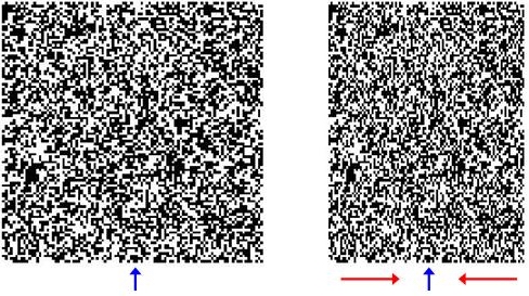
Suppose we create a random-dot stereogram that has zero disparity everywhere (i.e. the left and right images are identical) and then condense the right image uniformly in the horizontal direction, as suggested by the red arrows in the figure below. Based on your understanding of the geometry of the projection of points in space onto the left and right eyes, what would you expect observers to see when viewing this stereogram? To support your explanation, construct a diagram of the stereo projection geometry in this case, analogous to the exercises that you completed in lecture. For simplicity, you can assume that the central column of the left and right images projects to the same position in the left and right eyes, so that it has zero disparity, as suggested by the two blue arrows in the figure.

Problem 2 (25 points): The Marr-Poggio-Grimson Multi-resolution Stereo Algorithm

In class, we discussed a simplified version of the MPG multi-resolution stereo algorithm and performed a hand simulation of this algorithm on the board. This problem provides another example for you to hand simulate on your own. The zero-crossing locations are shown in the diagrams below. The top row shows zero-crossing segments obtained from a Laplacian-of-Gaussian operator whose central positive diameter is w = 8, and the bottom two rows show zero-crossing segments obtained from an operator with w = 4. Assume that the matching tolerance m (the search range) is m = w/2. In the diagram, the red lines represent zero-crossings obtained from the left image and the blue lines are zero-crossings from the right image (assume that they are all zero-crossings of the same sign). The axis below the zero-crossings indicates their horizontal position in the image.

Part a: Match the large-scale zero-crossing segments. In your answer, indicate which left-right pairs of zero-crossings are matched and indicate their disparities.

Part b: Match the small-scale zero-crossings, ignoring the previous results from the large-scale matching. In your answer, indicate which left-right pairs of zero-crossings are matched and indicate their disparities. Show your analysis for this case on the bottom row of the figure.

Part c: Match the small-scale zero-crossings again. This time exploit the previous results from the large-scale matching. Show your analysis for this case on the middle row of the figure.

Part d: What are the final disparities computed by the algorithm, based on the matches from Part c? The final disparity is defined as the shift in position between the original location of the left zero-crossings and the location of their matching right zero-crossings.

Part e: One of the constraints that is used in all algorithms for solving the stereo correspondence problem is the continuity constraint. What is the continuity constraint, and how is it incorporated in the simple version of the MPG stereo algorithm that you hand-simulated in this problem?

Problem 3 (45 points): Exploring a Region-Based Stereo Algorithm

The compStereo.m code file contains a function that implements a simple region based stereo corresondence algorithm, following the outline that we described in class. For each location in the left image, stereo disparity is computed by finding a patch in the right image at the same height and within a specified horizontal distance, which minimizes the sum of absolute differences between the right image patch and a patch of the same size centered on the left image location. The function records both the best disparity at each location and the measure of the sum of absolute differences that was obtained for this best disparity, and returns these values in two matrices (the function actually converts the match score to an average difference before returning the results, to reduce the magnitude of the values). There is a region around the perimeter of the image where no disparity values are computed. Carefully examine the code and comments to understand how it works, and how the various input parameters are defined.

The stereoScript.m file contains code to run an example of stereo processing for a visual scene containing a variety of objects at different depths. The left and right images are first convolved with a Laplacian-of-Gaussian operator to enhance the intensity changes in the images, and the convolution results are then supplied as the input images for the compStereo function. The parameter drange is the range of disparity to the left and right of the corresponding image location in the right image that is considered by the algorithm. nsize determines the neighborhood size; each side of the square neighborhood is 2*nsize + 1 pixels. The parameter border refers to the region around the edge of the image where no convolution values are computed. Finally, the parameter nodisp is assigned a value that is outside the range of valid disparities, and signals a location in the resulting disparity map where no disparity was computed. Carefully examine the code in stereoScript.m to understand all the steps of the simulation and display of the results.

Run the stereoScript.m code file and examine the results. In the display of the depth map, closer objects appear darker. Note that the value of nodisp is smaller than the minimum disparity considered, so locations where no disparity is computed will appear black. The results can be viewed with and without the superimposed zero-crossing contours. Where do errors occur in the results, and why do they occur in these regions of the image? You'll notice some small errors near the top of the image, where the original image has very little contrast. In areas such as this, the magnitude of the convolution values is very small and cannot be used reliably to determine disparity.

Modify the compStereo function so that it does not bother to compute disparity at locations of low contrast. A general strategy that can be used here is to first measure the average contrast within a square neighborhood centered on each location, and later compute disparity only at locations whose measure of contrast is above a threshold. The size of the neighborhood used to compute contrast can be the same as that used for matching patches between the two images. If the input images are the results of convolution with a Laplacian-of-Gaussian operator, the contrast can just be defined as the average magnitude of the convolution values within the neighborhood. Once the contrast is measured at each location (this can be stored in a matrix), determine the maximum contrast present in the image, and define a threshold that is a small fraction of that maximum contrast (e.g. 5%). Finally, revise the code for computing disparity so that it is only executed when the average contrast at a particular image location is above this threshold. Run the stereo code again - what regions are omitted from the stereo correspondence computation?

Examine how the results of stereo processing change as the size of the neighborhood used to define the left and right patches is changed (e.g. the neighborhood size, nsize, is increased to 25 pixels or decreased to 10 pixels). Explain why the results change as they do. Also describe what happens when the size of the convolution operator is increased (e.g. w = 8 pixels), and why.

For fun, modify the script to run the algorithm on the pair of stereo images named chapelLeft.jpg and chapelRight.jpg in the stereo folder, and report the mystery message that appears in the disparity map - you can change the parameters for this example to drange = 6 and nsize = 10. (For the original example, the image file names are left.jpg and right.jpg and initial parameters are drange = 20 and nsize = 20.) For this problem, submit your modified code files and answers to all the questions here.

Problem 4 (15 points): Multi-resolution Region-Based Stereo Algorithm

Using the ideas that were embodied in the multi-resolution stereo algorithm developed by Marr, Poggio, and Grimson, describe how the region-based stereo algorithm explored in Problem 3 could be modified to use multiple spatial scales. You can either consider the ideas embodied in the original multi-resolution stereo algorithm proposed by Marr and Poggio to account for the use of multiple spatial scales and eye movements in human stereo processing, or the simplified version of the Marr-Poggio-Grimson multi-resolution algorithm that you hand-simulated in Problem 2. You do not need to implement anything here, just describe a possible strategy in words.

Submission details: Hand in a hardcopy of your answers to these problems and your final compStereo.m and stereoScript.m code files. Please also submit an electronic copy of your code files by logging into the cs file server, connecting to your stereo folder and executing the following command:

submit cs332 assign2 *.*