|
CS 332
MATLAB Introduction |
|
Variables, vectors, and matrices
zeros and onescolon notation
matrix arithmetic and operations
other useful MATLAB functions:
sum, min, max,
             linspace, find
M-Files, scripts, directories, and the search path
MATLAB Apps and Live Scripts
Using the
help systemConditionals and loops
Aborting a computation and Command Window shortcuts
Managing variables and memory space
Defining new functions
using
help to obtain information about user-defined
functionsadding user input and output to function definitions
break and return statementsTypes of numbers
2D and 3D plotting
Working with images
image types
reading and writing images
displaying images
MATLAB is an extensive technical computing environment with advanced graphics and visualization tools and a rich high-level programming language, which is widely used for a variety of applications in academic, commercial, and government institutions. MATLAB is used heavily for modeling, empirical work, and data analysis in computer vision, neuroscience, psychology, and cognitive science, and has integrated Toolboxes that are especially useful for this work, including the Image Processing, Computer Vision, and Statistics and Machine Learning Toolboxes. This document introduces aspects of MATLAB that will be most useful for working with vision software in the course CS332 Visual Processing in Computer and Biological Vision Systems. To learn more about MATLAB, you can browse the extensive online help facility. The CS112 course website also contains links to additional MATLAB resources.
At Wellesley, MATLAB is available on the public Macs and PCs, and can be installed on your personal Mac or PC for use on or off campus. For more information about installing MATLAB on your laptop, go to this LTS MATLAB installation page. This platform road map at the MathWorks website provides useful information about the compatibility between MATLAB releases and operating system releases on various platforms. The MATLAB software is key-served, so there are a limited number of copies that can be used at one time, but this has not been a problem in the past. A student version of MATLAB can be purchased for $99.00 at the MathWorks website.
Starting MATLAB
To start MATLAB, double-click on the MATLAB_R2020a (or other version) icon, inside
the Applications folder on a Mac or accessible through the Start button
on a PC. Course materials, such
as images and code files, can be downloaded to a Mac or PC from the /home/cs332/download
directory on the CS file server using Cyberduck, or through
a zip file linked from the CS332 Schedule & Handouts page.
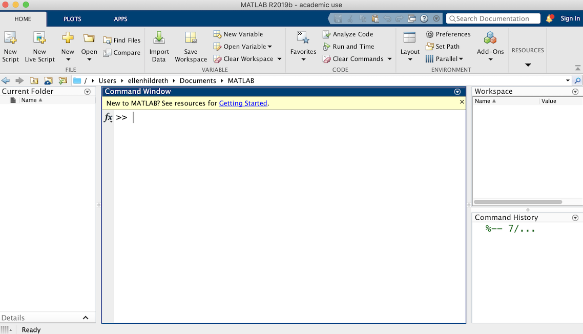
When you start MATLAB, a large window appears (the MATLAB desktop) that contains smaller windows that may include a Command Window, Command History, Current Folder, and Workspace window:
Layout menu that appears in the toolbar at the top of the MATLAB desktop.
Unlike languages such as Java and C, MATLAB is an interactive programming environment, in which the user types single commands at a prompt in the Command Window and the commands are executed immediately. The Command History window maintains a list of all of the commands entered in the Command Window during the current session. Double-clicking on any command in the Command History window evaluates this command again.
Immediately above the central Command Window is a pull-down menu with a text field that indicates the Current Folder (or Current Directory in older versions of MATLAB). The initial Current Folder will differ on Macs and PCs. Its contents are listed in the Current Folder window in the left region of the MATLAB desktop. The Workspace window lists the name, value, and type of all variables currently defined in the MATLAB workspace.
Variables, vectors, and matrices
When the MATLAB interpreter is waiting for a command from
the user, the command prompt >>
appears in the Command Window. Try entering the following commands that create some
variables and assign these variables to values. The printout below also shows the
MATLAB response (the phrases preceded by % are comments that should not be entered):
>> format compact         % removes extra vertical space from MATLAB printout
>> a = 10
a =
    10                    % MATLAB prints the value of each expression
>> b = [1 2 3]
b =                       % 1D vector of values
    1    2    3
>> c = [4 5 6; 7 8 9]
c =                       % 2D matrix of values - a semicolon separates row contents
    4    5    6
    7    8    9
>> d = [-1 0; 6 -7]
d =
   -1    0
    6   -7
>> e = [c d];             % semicolon at the end of a statement suppresses
>> e                             % the printout of its value
e =
    4    5    6    -1    0
    7    8    9     6   -7
MATLAB was originally designed to work efficiently with
large matrices of numbers, which are common in many science and engineering
applications. The name MATLAB is derived from MATrix LABoratory. A matrix is essentially an array of
numbers in one or more dimensions, although operations on matrices such as multiplication
follow certain mathematical rules. A 2D matrix with M rows and N columns is referred to as
an MxN matrix. In the above examples, the first variable, a,
is assigned to a single scalar
value that is stored in a 1x1 matrix. The variable b is assigned to a
row vector of three elements that are arranged horizontally. b
is represented as a 1x3 matrix. You can think of b as a
one-dimensional array. Brackets are used to enter the contents of a matrix, but
these brackets are not shown when the value is printed.
The variable c
is assigned to a 2x3 matrix that you can think of as a two-dimensional array.
In the assignment statement, the elements within each row are separated by
spaces (or optionally, commas) and the contents of the two rows are separated by a
semicolon. You can create a column vector in which the
elements are arranged vertically, by placing semicolons between the successive
elements, as in the following example:
>> f = [1; 2; 3]
f =
    1
    2
    3
The earlier assignment of the variable e
illustrates that new matrices can be formed out of
existing ones, by concatenating the parts. This assignment statement is also
terminated by a semicolon, which suppresses the printout of the returned
value. The value of a variable can be printed by typing the name of
the variable at the command prompt.
At any time, you can enter the clc command to clear the
Command Window.
The built-in size function returns the dimensions of a matrix:
>> size(b)           % returns a vector containing the two dimensions, 1x3
ans =
    1    3
>> size(e)
ans =
    2    5
>> size(e,1)         % note the optional second input - returns the first dimension
ans =
    2
>> size(e,2)         % returns the second dimension
ans =
    5
>> [rows, cols] = size(e)     % assigns dimensions to separate variables
rows =
    2
cols =
    3
When a value is returned, but not assigned to an explicit
variable name, the value is assigned to a default variable named ans. The
built-in function length returns the largest dimension of a matrix,
e.g. length(e) returns 5.
The elements of a 1D matrix can be accessed by specifying a single index in parentheses, while the elements of a 2D matrix can be accessed by placing two indices inside parentheses and separated by commas, as shown in the following examples:
>> b(2)
ans =              % indices begin with 1 (not 0, as in Python, Java, and C)
    2
>> d(2,2)
ans =
    -7
>> d(1,2)
ans =
    0
>> d(2,2) = 10     % assigning new contents to a matrix location
d =
   -1    0
    6   10
>> d(4,4) = 3
d =
   -1    0    0    0
    6   10    0    0
    0    0    0    0
    0    0    0    3
The last example shows that if a value is assigned to a matrix location that is outside the current bounds of the matrix, MATLAB automatically expands the matrix, padding it with zeros in locations where a value is not specified. When expanding the matrix, the old contents are copied to the new matrix, so this is not an efficient operation if performed many times.
zeros and ones
An initial matrix containing all 0's or all 1's can be created with the functions
zeros or ones, as shown in the following examples:
>> image1 = zeros(3,4)        % create a 3x4 matrix of zeros
image1 =
    0    0    0    0
    0    0    0    0
    0    0    0    0
>> image2 = ones(3,3)         % create a 3x3 matrix of ones
image2 =
    1    1    1
    1    1    1
    1    1    1
>> image3 = 5*ones(2,3)       % all matrix elements are scaled by 5
image3 =
    5    5    5
    5    5    5
>> image1D = 2*ones(1,6)      % to create a 1D matrix (vector) of zeros or ones,
image1D =                         % you still need to specify two dimensions
    2    2    2    2    2    2
The zeros and
ones functions can also be used
to create 3D matrices. This is illustrated in the following example, which also
shows how to access the dimensions and elements of a 3D matrix:
>> image3D = zeros(10,10,3);
>> [xdim ydim zdim] = size(image3D)
xdim =
    10
ydim =
    10
zdim =
    10
>> image3D(3,6,2) = 100;
colon notation
It is often desirable to create a set of equally spaced
numbers or access a range of indices in a matrix all at once. A range of
numbers can be specified using colon notation.
The expression a:b
denotes a sequence of consecutive numbers from a
to b, incrementing by 1. The
expression a:b:c denotes a
sequence of numbers from a to c, changing by b.
In the following examples, some sample sequences of
numbers are placed in 1D matrices:
>> g = 2:6
g =
    2    3    4    5    6
>> h = 3:2:11
h =
    3    5    7    9    11
>> k = 2:-1:-3
k =
    2    1    0    -1   -2   -3
>> m = 0.2:0.4:2.2
m =
    0.2000   0.6000   1.0000   1.4000   1.8000   2.2000
The last example created a matrix of floating point numbers, and by default,
MATLAB prints these numbers with 4 digits after the decimal point.
Colon notation can be used to specify a range of indices for a matrix. Inside a
matrix reference, a single colon by itself specifies an entire row or column. The
keyword end inside a reference to the indices of a matrix
specifies the upper limit of a particular dimension. The following
examples illustrate these concepts:
>> e
e =
    4    5    6   -1    0
    7    8    9    6   -7
>> e(1,2:4)
ans =                   % row 1, column indices 2 through 4
    5    6   -1
>> e(1:2,4:5)
ans =                   % rows 1 and 2, columns 4 and 5
   -1    0
    6   -7
>> e(:,2)
ans =                   % all rows in column 2
    5
    8
>> e(2,:)
ans =                   % all columns in row 2
    7    8    9    6   -7
>> e(1,3:end)
ans =                   % row 1, from column 3 to the last column
    6   -1    0
>> e(:,3) = 0           % assign all rows in column 3 to zero
e =
    4    5    0   -1    0
    7    8    0    6   -7
The contents of one matrix can be copied into another, using colon notation to specify regions of the matrices:
>> im1 = zeros(5,5)
im1 =
    0    0    0    0    0
    0    0    0    0    0
    0    0    0    0    0
    0    0    0    0    0
    0    0    0    0    0
>> im2 = ones(3,3)
im2 =
    1    1    1
    1    1    1
    1    1    1
>> im1(2:4,3:5) = im2           % copy all of im2 into im1, starting at
im1 =                              % row 2, column 1 of im1
    0    0    0    0    0
    0    0    1    1    1
    0    0    1    1    1
    0    0    1    1    1
    0    0    0    0    0
>> im1(4:5,1:2) = im2(1:2,1:2)   % copy a subregion of im2 into im1
im1 =
    0    0    0    0    0
    0    0    1    1    1
    0    0    1    1    1
    1    1    1    1    1
    1    1    0    0    0
>> subimage = im1(2:4,1:3)      % create a separate matrix that is a
subimage =                               % subregion of im1
    0    0    1
    0    0    1
    1    1    1
matrix arithmetic and operations
If two matrices have the same dimensions, their contents can be added, subtracted, multiplied, and divided on an element-by-element basis:
>> a1 = [2 6 3; 0 4 7; 1 5 8]
a1 =
    2    6    3
    0    4    7
    1    5    8
>> a2 = [6 4 1; 2 8 0; 3 7 5]
a2 =
    6    4    1
    2    8    0
    3    7    5
>> a1+a2            % add elements at corresponding locations of a1 and a2
ans =
    8   10    4
    2   12    7
    4   12   13
>> a1-a2            % subtract corresponding elements of a1 and a2
ans =
   -4    2    2
   -2   -4    7
   -2   -2    3
>> a1.*a2           % multiply corresponding elements of a1 and a2
ans =                    % note the period before the * symbol!
   12   24    3
    0   32    0
    3   35   40
>> a2./a1           % divide elements of a2 by corresponding elements of a2
ans =                       % note: division by 0 does not generate an error!
   3.0000   0.6667   0.3333
      Inf   2.0000        0      % Inf represents infinity (undefined)
   3.0000   1.4000   0.6250
>> a1./a2           % divide elements of a1 by corresponding elements of a2
ans =
    0.3333   1.5000   3.0000
         0   0.5000      Inf
    0.3333   0.7143   1.6000
>> 2*a1             % scale all the elements by 2 (a1 does not change)
ans =
    4   12    6
    0    8   14
    2   10   16
>> a1.^2            % square all the elements (a1 does not change)
ans =
    4   36    9
    0   16   49
    1   25   64
>> a1*a2            % perform a real matrix multiplication
ans =
   33   77   17
   29   81   35
   40  100   41
>> a1^2             % multiply a1 by itself using matrix multiplication
ans =
    7   51   72
    7   51   84
   10   66  102
In each of the above examples, a new matrix was created and automatically
assigned to the temporary variable ans. To reassign a variable to
the new matrix, or assign the result to a new variable name, the expression
must be embedded in an assignment statement, e.g. a3 = a1 + a2.
other useful MATLAB functions: sum, min, max, linspace, find
Some additional built-in MATLAB functions that will come in
handy include sum, min, max, linspace, and find, illustrated
in the following code:
>> test1D = [3 5 1 7];
>> sum(test1D)       % returns the sum of the contents of a 1D matrix
ans =
    16
>> test = [1 2 3; 4 5 6; 7 8 9]
test =
    1    2    3
    4    5    6
    7    8    9
>> sum(test)         % for a 2D matrix, sum returns a 1D matrix of
ans =                   % the sums of the values in each column
   12   15   18
>> sum(sum(test))    % invoke sum twice to obtain the sum of all the
ans =                   % contents of a 2D matrix
   45
>> min(test1D)       % returns the minimum value in a 1D matrix
ans =
    1
>> min(test)         % returns vector of minimum values in each column
ans =
    1    2    3
>> min(min(test))    % returns the minimum value in a 2D matrix
ans =
    1
>> max(test1D)       % returns the maximum values
ans =
    7
>> max(test)
ans =
    7    8    9
>> max(max(test))
ans =
    9
linspace(x1,x2,n) returns
a 1D matrix containing n values
that are evenly spaced between x1
and x2:
>> linspace(2,15,5)
ans =
   2.0000   5.25000   8.5000   11.7500   15.0000
Finally, the find
function returns the locations (indices) of values in a matrix that satisfy an input
logical expression:
>> nums = rand(1,7)      % create a 1D matrix of random numbers between 0 and 1
nums =
   0.9355   0.9169   0.4103   0.8936   0.0579   0.3529   0.8132
>> find(nums>0.5)        % returns the indices of numbers larger than 0.5
ans =
    1    2    4    7
>> nums = rand(4,4)      % create a 2D matrix of random numbers
nums =
   0.0099   0.6038   0.7468   0.4186
   0.1389   0.2722   0.4451   0.8462
   0.2028   0.1988   0.9318   0.5252
   0.1987   0.0153   0.4660   0.2026
                             % find numbers between 0.33 and 0.67
>> [r, c] = find((nums > 0.33) & (nums < 0.67))
r =                      % r is a column vector of the row coordinates
    1                         % of numbers in this range
    2
    4
    1
    3
c =                      % c is a vector of the column coordinates
    2                         % of numbers in this range
    3
    3
    4
    4
The two vectors r and c indicate that there are
numbers between 0.33 and 0.67 at (row, column) locations (1,2), (2,3), (4,3), (1,4), and (3,4).
An implication of the above examples is that a conditional expression like
(nums > 0.5) can be applied to an entire vector or matrix of values all
at once. This expression returns a vector or matrix of logical values 1 and 0
that represent true and false, respectively. For example:
>> test = [1 2 3; 4 5 6; 7 8 9];
test =
    1    2    3
    4    5    6
    7    8    9
>> odds = (rem(test,2) == 1);    % rem is the remainder function
odds =
    1    0    1
    0    1    0
    1    0    1
For more information about these and other MATLAB functions,
see the section on Using the A sequence of MATLAB commands can be stored in a file
and executed by entering the first name of the file in the Command Window.
The file must have a filename extension of An existing M-file can be opened in the MATLAB editor through the In this case, the Multiple files can be open in the editor at one time - the files are overlaid and
can be selected by clicking on the tab with their name near the top of the editor window. You can
type commands in the editor, and the code will be formatted automatically with indentation
to make the code more readable. A code file can be saved by clicking on the floppy disk icon labeled Suppose a file is created, named A comment can be placed in an M-File by preceding the text
with A script is executed as if the individual commands were
entered, one-by-one, in the Command Window. As a consequence, existing
variables in the MATLAB workspace can be altered by a script that uses
variables of the same name, and new variables created by a script will remain
in the workspace after execution is complete. In the Starting MATLAB section, it was noted that there is
a default Current Folder whose pathname differs on Macs and PCs.
The folder whose contents are listed in the Current Folder window can be
changed. The menu bar directly above this window contains arrow and folder icons for
navigating up and down the directory tree. Alternatively, you can select the desired
folder using the pull-down menu above the central Command Window.
In the Command Window, the When a name, such as The search path initially contains all the folders
where MATLAB stores its files. The search path can be viewed by selecting
In order to execute a script from the editor or by entering the name of the script in the Command
Window, the script file must be stored in the Current Folder or some other
folder listed on the search path. When naming variables and files, it is helpful to remember
the procedure that MATLAB uses to resolve a name that appears in a script or is
entered directly in the Command Window. To determine whether a particular name
already exists, use the The MATLAB App Designer tool enables
users to create interactive programs with graphical user interfaces. In CS332, several demonstration programs
are written as interactive apps. The code files for these apps have a file extension of
MATLAB has an extensive library of built-in functions that are documented through the The The comments can then be accessed through the Command Window: You can also search for information through the search box at the top of the
MATLAB desktop. MATLAB provides The expressions in the above patterns are logical
expressions that can be created using the following relational operators,
similar to Python, Java, and C: The general pattern for the It is common to use the colon operator or an existing 1D
matrix to specify the values for the variable that controls the number of times
that the body of the loop is executed. The following examples
illustrate the use of Suppose the above statements were saved in an M-File named
Now that you know about loops, it's useful to know how to
terminate a runaway computation. When MATLAB is busy performing a computation,
the word When entering commands in the Command Window, there are a
number of handy shortcuts available. The up-arrow and down-arrow keys cycle
up and down through previously
entered commands, allowing you to repeat the execution of a command. The left-
and right-arrow keys move the cursor back and forth through a line to
facilitate editing, and the Tab key can be used for command completion. If you
type part of a command and decide not to execute this command, press the escape
key to erase the line. A final handy shortcut is that multiple commands can be typed on one line,
separated by commas (although this can lead to less readable code): Large 2D and 3D matrices can occupy substantial memory space.
It is possible for MATLAB to run out of memory, making it impossible to do
further work. Fortunately, existing variables that are no longer needed can be
eliminated, freeing up memory space for new variables. The
Executing the command A new function can be defined in an M-File whose first
file name is the same as the name of the function. To open a file to define a new function,
select Consider the following function named This function must be stored in a file named When a function is called with a particular set of inputs,
the values of these inputs are copied into the input variables specified in the
declaration line of the function definition. Similarly, values returned by a
function are copied into the variables specified in the function call. Local
variables created within a function definition only exist during the execution
of the function. The following examples illustrate a variety of function
definitions and their application. The function The function The last two functions can be invoked as follows: The Here is an example of its use:
The following function returns a blurry version of an input image, combining
a number of ideas described earlier:
An M-File that contains a new function definition can also
contain the definitions of other functions that serve as helper functions, but
only the main function whose name is the same as the M-File can be called
directly from the Command Window or by functions in other M-Files. It was mentioned earlier that the It is common to place a comment immediately following the
header that illustrates how the function is invoked, so that this information
is also accessible through the A function can request input from the user with the When concatenating multiple strings to print with The execution of a By default, MATLAB represents numbers as double-precision
floating point numbers that each require 8 bytes of storage space. A large 2D
or 3D matrix of double-precision floating point numbers occupies a lot of memory
space! Fortunately such precision is often not needed and MATLAB provides
several other types of numbers that can be represented more compactly: For each type, there is a function of the same name that
converts an input number to the desired type. In the example below, the
function The When printing floating point numbers of type Note: When computations are performed on matrices that are integer
types, the results are converted to the same integer type, as shown in the following
examples, which convert all results to the The By default, the Multiple plots can be displayed within a single figure window using the
3D plots can be created with the functions
Pictures with arrows can be created with the When many figure windows are open, displaying plots or images, the memory storage
for all of these windows sometimes interferes with the memory space used for numerical
computations, producing erroneous results. For this reason, you should not have too
many figure windows open at one time! Individual figure windows can be closed by
clicking on the close button in the upper right corner of the window. All of the current
windows can be closed at once by executing the following command: You can learn much more about all of the plotting
functions through the MATLAB The basic MATLAB system, combined with the Image Processing
Toolbox, provides many functions for reading, writing, displaying and
processing 2D and 3D images. This section introduces the basic facilities that
we will use extensively in CS332. There are four types of images that are supported in MATLAB.
A binary image contains only black and white pixels and is stored in a logical matrix
of 0's and 1's. An indexed image is a matrix of integers in
a range from 1 to n that each represent an index into a separate colormap.
The colormap is stored in an
nx3 matrix, where each row contains values for the red, green and blue
components of a particular color. Indexed images can be stored in matrices of
type MATLAB can read and write images using many different file
formats, obtained from a variety of sources. The most common image file types
that we will use are JPEG and PNG. The functions for reading and writing
images are The By default, the image is stored in the Current Folder. MATLAB provides two functions for displaying images,
By default, the Multiple images can be displayed in separate figure windows by calling the
The You can zoom in and out of the image to view it at different
resolutions, and navigate around the image with the mouse. Expand
the Pixel Region Tool window with the mouse to view intensity or RGB
values over a larger image region.
RGB color images can be
converted to gray-level images using the As noted earlier, when displaying any gray-level image with Again, if empty brackets are provided as the second input, The windows created with
Documentation for the Image Processing Toolbox, available online through
the Throughout the course, we will use a mixture of built-in functions from the basic MATLAB system,
additional functions from Toolboxes such as the Image Processing, Computer Vision, or Statistics
and Machine Learning Toolboxes, and custom-built software for analyzing images. Most of the
basic MATLAB facilities that you will use are introduced in this document, and
other tools will be presented as needed.help system. Other
built-in functions
that may appear in course software include abs, exp, sqrt, prod, mean, fix, round, rem,
sin, cos, and tan.
M-Files, scripts, directories, and the search path
.m and is referred to
as an M-File. One type of M-file is a script. Although any
text editor can be used to create an M-File, MATLAB provides its own editor
that is convenient to use. There are at least three ways to open an initial editor window
to start a new script:
edit in the Command Window
New Script icon near the upper left corner of the MATLAB window
Script from the New menu to the right of the
New Script icon
Open menu
near the upper left corner of the MATLAB window, or by clicking on the folder above this menu.
You can also double-click on the file name in the Current Folder window, or
invoke the edit command in the Command Window, for example:
edit myCodeFile
myCodeFile.m file must be stored in the Current
Folder, or exist somewhere on MATLAB's search path described later in
this section.Save along
the top of the editor window, or through the Save menu below this icon.
When a file is first created, a dialog box will appear where the name
of the file can be entered. Either type the full file name (e.g. myCodeFile.m) or first
file name (e.g. myCodeFile) in the text box
labeled Save As: and click on the Save button. Unless otherwise specified,
the file will be stored in the Current Folder.testFile.m.
The sequence of commands in this file can then be executed by entering the name
testFile in the Command Window. From the editor, the script can also be run by
clicking on the green arrow along the top menu bar.%, as shown in the above
code samples. Multiple lines of text can be put in comments by surrounding the
block of text with %{ and %} placed on separate lines, as shown
in the following script:%{
This script creates a simple image with
two patches of constant intensity against
a black background
%}
image = zeros(50,50);
image(10:20,10:30) = 100;
image(25:40,15:45) = 200;
cd command can also be used to specify
a Current Folder.
testFile,
is entered in the Command Window, the MATLAB interpreter first checks if there
is a variable of this name in the workspace. If not, it checks whether there is
a built-in function of this name. If no built-in function exists, it looks for
an M-File in the Current Folder with this name as the first file name (i.e.,
testFile.m). If no such file is
found, the interpreter checks each folder in a list called the search path for a file of this name. If
no file is found on the search path, an error is generated. Set Path from the menu bar at the top of the MATLAB window.
This brings up a dialog box with a list of folders that are currently
on the search path. On a Mac or PC, a new folder can be added by
clicking either the Add Folder... or Add Folder with Subfolders...
button, which brings up another dialog box that can be used to navigate to the
folder to be added to the search path.
exist
function, which returns 0 if a name does not exist:>> exist magic % there's a file magic.m on MATLAB's search path
ans =
2
>> exist stars % the name 'stars' does not exist
ans =
0
MATLAB apps and Live Scripts
.mlapp. In addition, users can create
MATLAB Live Scripts
that integrate text, figures, and MATLAB code boxes where code can be modified and executed (similar to
Python Notebooks). Some of the CS332 class activities will use Live Scripts, which have a file extension of
.mlx. For CS332, you do not need to know how to create apps or Live Scripts, but may be interested
in learning about them through the MATLAB documentation.
Using the help system
help
system. Just enter help or doc
followed by the name of a function:>> help exist
...
>> doc magic
help
command can also be used to print information about user-defined scripts and
functions. In the case of scripts, any comments at the top of the script file
that are preceded with a % are
printed. For example, suppose the following script were stored in a file named
helpTest.m:% this script illustrates the application of the
% help command to user-defined script files
a = 10;
b = 3;
>> help helpTest
    this script illustrates the application of the
    help command to user-defined script files
Conditionals and loops
if
and switch statements for
conditionals, and for and while statements for loops. This
section introduces if and for statements. The if
statement can follow one of three patterns:if conditional-expression
<commands to evaluate if true>
end
if conditional-expression
<commands to evaluate if true>
else
<commands to evaluate if false>
end
if conditional-expression1
<commands to evaluate if conditional-expression1 is true>
elseif conditional-expression2
<commands to evaluate if conditional-expression2 is true>
elseif conditional-expression3
<commands to evaluate if conditional-expression3 is true>
...
else
<commands to evaluate if all conditional expressions are false>
end
> < >= <= == ~= & | && ||
(note that == is used to test for equality - the single equals = is used only
for assignment).
for statement is:for variable = values
<commands to evaluate for each value of variable>
end
if and for
statements. The statements are
formatted as they would appear when entered into an M-File in the editor. Semicolons
are typed at the end of each assignment statement so that the MATLAB output is
suppressed during execution:randomNums = rand(1,7); % create a 1D matrix of random numbers
numbers = zeros(1,7); % between 0.0 and 1.0
for i = 1:7 % loop is executed 7 times, with i assigned
if (randomNums(i) < 0.33) % to consecutive integers from 1 to 7
numbers(i) = 0;
elseif (randomNums(i) < 0.66)
numbers(i) = i;
else
numbers(i) = 1;
end
end
for i = 1:3:7 % loop is executed 3 times, with i assigned
numbers(i) = numbers(i) + 100; % to 1, 4 and 7
end
numbers2D = rand(3,6);
for i = 1:3 % nested for statements can be used to loop
for j = 1:6 % through a 2D matrix
if numbers2D(i,j) < 0.5) | (j == 3)
numbers2D(i,j) = 0.0;
end
end
end
nums = [3 8 2 9 1 5 8];
sum = 0;
for val = nums % loop is executed 7 times, with val assigned
sum = sum + val; % to each of the 7 numbers stored in nums
end
forTest.m and then executed in the Command
Window. An example of the final values stored in the variables randomNums,
numbers, numbers2D, and sum is shown in the following printout:>> randomNums
randomNums =
0.6992 0.7275 0.4784 0.5548 0.1210 0.4508 0.7159
>> numbers
numbers =
101 1 3 104 0 6 101
>> numbers2D
numbers2D =
0.8928 0.8656 0 0 0 0
0 0 0 0 0.8439 0.9943
0 0.8049 0 0.6408 0 0
>> sum
sum =
36
Aborting a computation and Command Window shortcuts
Busy is printed in the
lower left corner of the full MATLAB window. The execution of any command can
be aborted by typing control-C.>> x = 10, y = 15, z = sqrt(x^2 + y^2)
x =
10
y =
15
z =
18.0278
Managing variables and memory space
who command prints the names of all
variables currently defined in the MATLAB workspace, the
whos command prints the name, size and
type of each variable, and the clear
command deletes variables from the workspace: >> whos
Name Size Bytes Class
ans 1x1 8 double
im1 10x10 800 double
im2 20x20 3200 double
image 50x50 20000 double
>> clear im1 im2
>> who
Your variables are:
ans image
clear all deletes all variables from the workspace.Defining new functions
Function from the New menu near the top of the MATLAB
window, and the skeleton of a function definition will appear in the MATLAB editor.
The first statement in the file is a declaration line that
indicates the name of the function and its inputs and outputs. This declaration
line implicitly shows the format for calling the function. The generic pattern
for a function definition is:function <outputs> = <function name> (<inputs>)
<statements comprising the body of the function>
<inputs>
is a list of input variable names, separated by commas. Inside the body of the
function, the inputs can be accessed by name and assigned to new values. If the
function returns a single value, then <outputs>
is a single variable name. If multiple values are returned, then <outputs>
is a bracketed list of
variable names, separated by commas. Inside the body of the function, the
output variable name(s) must be assigned to the value(s) to be returned. In recent versions of
MATLAB, the initial function skeleton contains an end statement at the end of the
function, but this is not essential. gaussian:function g = gaussian(x, sigma)
% returns the value of a Gaussian function for
% a particular input location and spread
g = exp(-1.0*(x^2/sigma^2);
gaussian.m. The follow examples
show how this function can be called:>> gval = gaussian(3.0,2.0)
gval =
0.1054
>> gvals = zeros(1,6)
gvals =
0 0 0 0 0
>> for x = 0:5
gvals(x+1) = gaussian(x,2.0); % the body of a for statement is not indented
end % when entered directly in the Command Window
>> gvals
gvals =
1.0000 0.7788 0.3679 0.1054 0.0183 0.0019
gaussianFun
returns a 1D matrix of samples of a Gaussian function. Its definition
illustrates the reassignment of an input variable, sigma, and use
of a local variable, xvals:function g = gaussianFun(range, numSamples, sigma)
% returns a 1D matrix of samples of a Gaussian function with spread
% specified by sigma and x ranging from -range to +range
sigma = -1.0/sigma^2;
xvals = linspace(-range, range, numSamples);
xvals = xvals.^2;
g = exp(sigma.*xvals);
gaussianPlot
illustrates the format of a declaration line for a function with no inputs and
outputs. The plot function is
described in the section, 2D and 3D plotting.function gaussianPlot
% function with no inputs and outputs, displays a graph of a gaussian function
gauss = gaussianFun(4,9,2.0); % call another user-defined function
xcoords = [-4:4];
plot(xcoords,gauss);
>> gauss = gaussianFun(4,9,2.0)
gauss =
  Columns 1 through 7
    0.0183   0.1054   0.3679   0.7788   1.0000   0.7788   0.3679
  Columns 8 through 9
    0.1054   0.0183
>> gaussianPlot
findZeros function defined below returns two values, a 2D matrix and a number:function [zeroMap, numZeros] = findZeros(image)
% returns a 2D matrix that is the same size as the input image matrix, with
% 1's % at the locations of the zero values in the input image and 0's
% elsewhere. also returns the number of zeros in the input image
[xdim ydim] = size(image); % get the dimensions of the input matrix
zeroMap = zeros(xdim,ydim); % createa new matrix of the same size
[x y] = find(image==0); % find the locations of zeros in the image
numZeros = length(x); % determine the total number of zeros
for i = 1:numZeros % place 1's at the corresponding locations
zeroMap(x(i),y(i)) = 1; % of the zeroMap matrix
end
>> testImage = [6 2 0 6 1; 0 7 2 5 0; 7 6 2 0 3; 6 1 0 3 7; 8 0 6 9 0]
testImage =
    6    2    0    6    1
    0    7    2    5    0
    7    6    2    0    3
    6    1    0    3    7
    8    0    6    9    0
>> [zMap, nZeros] = findZeros(testImage)
zMap =
    0    0    1    0    0
    1    0    0    0    1
    0    0    0    1    0
    0    0    1    0    0
    0    1    0    0    1
nZeros =
    7
function newImage = fuzzy(image,nsize)
% returns a blurry version of the input image (a 2D 8-bit (uint8) matrix),
% where the intensity at each image location is replaced by an average of
% its neighbors within an area that covers nsize rows and columns on both
% sides of each location

% convert to double to enable floating-point calculation of average
image = double(image);
[rows,cols] = size(image);       % create a new image of the same size
newImage = zeros(rows,cols);
% scale factor used to divide the sum of intensities in each neighborhood
% by the number of pixels in the neighborhood
scale = 1.0/((2*nsize+1)^2);
% compute average intensity at each location, omitting a border of nsize
% pixels from the computation
for row = nsize+1:rows-nsize
    for col = nsize+1:cols-nsize
        newImage(row,col) = ...
            scale*sum(sum(image(row-nsize:row+nsize,col-nsize:col+nsize)));
    end
end
newImage = uint8(newImage);      % return an 8-bit image
using
help to obtain information about user-defined functionshelp command can be used to obtain information
about user-defined functions. In this case, any comment lines that immediately follow
the function header and appear with a %
at the beginning of the line are printed:>> help gaussian
returns the value of a Gaussian function for
a particular input location and spread
help
command, for example:function g = gaussian(x, sigma)
% g = gaussian(x, sigma)
% returns the value of a Gaussian function ...
adding user input and output to function definitions
input function, which
has a single input that is a quoted text string that is printed as a prompt to the user. The
simplest ways to print out intermediate values during the execution of a
function are to omit the semicolon at the end of an assignment statement, or
to create a string that contains text and variables, as illustrated in the
newGaussian function shown below. The
disp function displays in input value
without printing a variable name. In the first call to disp,
the input is an vector of characters created by
concatenating two literal strings and a string representation of the number
stored in sigma, created with
the num2str function. function g = newGaussian(x)
% returns a sample of a Gaussian function after prompting the user for a value
% for sigma. also illustrates ways to provide printout of intermediate values
sigma = input('enter a value for sigma: '); % request user input
disp(['you entered ' num2str(sigma) ' at the prompt']);
disp('the resulting Gaussian value is');
g = exp(-1.0*(x^2/sigma^2)) % note omission of semicolon at the end
disp('have a nice day!');
>> gval = newGaussian(2);
enter a value for sigma: 3.0
you entered 3 at the prompt
the resulting Gaussian value is
g =
0.6412
have a nice day!
disp,
square brackets are used to combine the components of the string. To create nicely formatted
output, explore the sprintf and fprintf functions, similar to their
counterparts in C and C++. break and return statementsbreak statement inside a loop immediately terminates the loop.
The execution of a return statement anywhere in a
function immediately terminates the function.Types of numbers
MATLAB name    size(bytes)      description
uint8             1             integers 0 to 255
uint16            2             integers 0 to 65,545
uint32            4             integers 0 to 4,294,967,295
int8              1             integers -128 to 127
int16             2             integers -32,768 to 32,767
int32             4             integers -2,147,483,648 to 2,147,483,647
single            4             single-precision floating point
uint8 is used to create
a matrix of integers of type uint8
from a matrix of numbers of type double:>> image = 200*ones(100,100);
>> newImage = uint8(image);
>> whos
Name Size Bytes Class
ans 1x1 8 doubl
image 100x100 80000 double
newImage 100x100 10000 uint8
newImage matrix can be created directly, without the intermediate
image matrix, by executing the statement
newImage = uint8(200*ones(100,100)).double, MATLAB uses
scientific notation to print very large or very small numbers, as shown here:>> number = 1230000000
number =
1.23e+09
>> number = 0.000789
number =
7.8900e-04
uint8 type (integers between
0 and 255):
>> nums1 = uint8([100 10 200]);
>> nums2 = nums1 + 100
nums2 =
   200   110   255
>> nums3 = nums1 - 100
nums3 =
     0     0   100
>> nums4 = nums1/100
nums4 =
   1   0   2
>> whos
  Name       Size      Bytes  Class
  nums1      1x3           3  uint8
  nums2      1x3           3  uint8
  nums3      1x3           3  uint8
  nums4      1x3           3  uint8
2D and 3D plotting
plot function can be used to create 2D graphs. The essential inputs to
plot are two 1D matrices containing the x and y coordinates of the points to be
plotted. The plot function opens a graphic window called a figure
window, draws axes with labels that are scaled to fit the range of the data, and connects the
points with straight lines, as shown in the following example:>> xc = 0.0:0.1:2*pi; % 1D matrix of evenly spaced x coords from 0 to 2π
>> yc = sin(xc); % 1D matrix of samples of a sine function
>> plot(xc, yc); % plot function displays the graph shown below

plot function draws a new graph in the most recently opened
figure window. To create a new window, execute the figure
command. The plot function is
extremely versatile. For example, you can change the appearance and range of
the axes, adjust the appearance of the graph with different line types, symbols
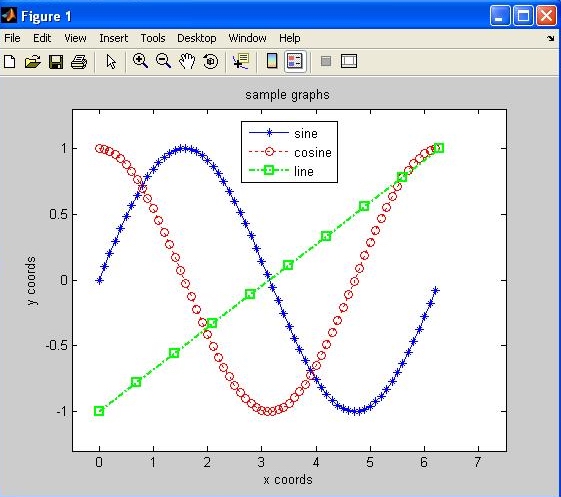
and colors, add labels and legends, and display multiple graphs superimposed.
Some of these facilities are illustrated below:xc = 0.0:0.1:2*pi;
yc = sin(xc);
yc2 = cos(xc);
plot(xc, yc, 'b-*')
hold on
plot(xc, yc2, 'r:o')
plot(linspace(0,2*pi,10), linspace(-1,1,10), 'g-.s', 'LineWidth', 2)
axis([-0.5 7.5 -1.3 1.3])
xlabel('x coords')
ylabel('y coords')
title('sample graphs')
legend('sine', 'cosine', 'line', 'Location', 'Best')
hold off
subplot command, and scatter plots can be created with the
scatter function. The contents of
figure windows can also be saved for later retrieval or insertion into
documents by selecting the Save or Save As... options from
the File menu at the top of the figure window.plot3, scatter3, mesh
and surf. The following example
illustrates the creation of a surface plot:>> [x,y,z] = peaks(30); % peaks returns x,y,z coordinates of a surface
>> surf(x,y,z); % creates the 3D surface plot shown below

quiver function, for example, to
illustrate how features are moving in an image:
>> close allhelp facility.Working with images
image types
uint8, uint16 or double. The colormap is always a
matrix of type double. An intensity image consists of intensity,
or gray-scale values. When displayed, an intensity image appears as a black and
white photograph. Intensity images can be stored in matrices of type uint8, uint16 or
double. Finally, an RGB image, or truecolor image, is stored
in an mxnx3 matrix. The first two dimensions represent pixel location and the
third dimension specifies the red, green and blue components for the color of
each image pixel. An RGB image can also be stored in matrices of type uint8, uint16
or double. We will primarily work with
intensity and RGB images. It is easy to convert between image types, using
functions that were mentioned briefly in the section,
Types of numbers. MATLAB also provides specific functions such
as rgb2gray that converts an RGB image into a gray-level image.reading and writing images
imread and imwrite, which are defined in the
Image Processing Toolbox. Extensive information about
various image file formats and their specification can be obtained through the
help pages for these two functions.
The imread function has one
essential input that is the name of the image file to be loaded into the MATLAB
workspace. Often MATLAB can infer the type of file from its contents, so that
it is not necessary to provide any further inputs to the imread function:>> coins = imread('coins.png');
>> peppers = imread('peppers.png');
>> whos
Name Size Bytes Class
coins 246x300 73800 uint8
peppers 384x512x3 589824 uint8
imfinfo function prints information about the format of an image, for
example, try entering imfinfo('coins.png'). The
essential inputs to the imwrite
function are the image name and file name, with a file name extension that
indicates the file format to use:>> imwrite(image1, 'image1.jpg');
>> imwrite(image2, 'image2.png');
displaying images
imshow and imtool, which are also defined in the Image
Processing Toolbox.>> imshow(coins);

imshow
function displays the image using 256 discrete levels of gray. The number of
gray levels can be changed by providing a second integer input, e.g.
imshow(coins,64). In the case of an
8-bit image, the value 0 is normally displayed as black and 255 is displayed as
white. The imshow function can
be called with a specified range of intensities to be displayed from white to
black. For example, imshow(coins,
[50,200]) displays intensity values of 50 or less as black, and
intensities of 200 or higher as white. The values between 50 and 200 are evenly
spread over the levels of gray from black to white. imshow
can also be used to display binary, indexed and
RGB images. If the input image is of type double, MATLAB assumes
that the values to be displayed range from 0.0 to 1.0. In this case, any values
below 0.0 are displayed as black, values above 1.0 are shown in white, and values
between 0.0 and 1.0 are displayed as shades of gray. Again, a different range of
intensities can be specified, e.g. imshow(newImage,[1.0,5.0]).
If empty brackets are provided as a second input, MATLAB will use the actual minimum
and maximum intensity values in the image as the range to be displayed from
black to white, e.g. imshow(image,[]).
figure function to create a new window. Keep in mind that MATLAB
can become confused if too many figure windows are open, so be sure to close
unnecessary windows, either individually or with the close all
command. Using the subplot
function, multiple images can be displayed inside a single figure window. You
can zoom in or out of an image displayed in a figure window, or change the size
of the image by changing the window size. It is also possible to add figure
annotations and print images that are displayed with imshow.imtool
function displays the image in a separate window called an Image Tool. The
Image Tool provides special tools for navigating around large images and inspecting
small regions of pixel values. Similar to imshow,
a particular range of intensity values can be specified when calling imtool,
e.g. imtool(coins, [50,200]). The main Image Tool window has a
menu bar that allows you to open a smaller Overview window containing the full
image, and a Pixel Region window that displays the intensity or RGB values within
small image regions:>> imtool(coins);

>> imtool(peppers);

rgb2gray function:>> pepper2 = rgb2gray(peppers);
>> imshow(pepper2);

imshow or
imtool, a second
input can be provided that specifies a desired minimum and maximum intensity to display
as the darkest and lightest shades of gray in the display. In the following example,
the minimum and maximum intensities are set to 100 and 200, respectively:
>> imshow(pepper2,[100,200]);
imshow(pepper2,[]),
then the actual minimum and maximum intensity values in the image are used for
display. Beware! By default, if a second input is not provided to imshow
or imtool, MATLAB assumes that an image stored in a double type matrix has
values in the range [0,1], and an image stored in a uint8 type matrix has values in the
range [0,255].
imtool can be closed all at once by executing the following command:>> imtool close all
Help menu, provides more detailed information about how to use the Image Tool.