Jupyter Notebook with sckernel Demo

The following short notebook demonstrates a few of the features of integrating SuperCollider with Jupyter Notebook.

1. SuperCollider as a Calculator

The following expressions can be evaluated by SuperCollider just like a calculator. Most of your intuitions about the following code apply. To see the output of the code, check the post window that was automatically started at the startup of this notebook.

3 + 4

3 / 2

2.5 * 1

2. AM Modulation

First start up the SuperCollider audio server.

s.boot; // Wait for the server to boot up

I can write equations and then test out what those sound like in SuperCollider. Jupyter Notebooks can display nicely formatted mathematical equations which is useful when teaching digital signal processing.

$$A_1\sin(2\pi f_1t + \phi_1)A_2\sin(2\pi f_2t + \phi_2)$$

// A SuperCollider implementation of the above equation

SynthDef(\am, {
    arg a1 = 0.1, f1 = 100, p1 = 0, a2 = 0.1, f2 = 200, p2 = 0;
    var sig;
    
    sig = SinOsc.ar(f1, p1, a1) * SinOsc.ar(f2, p2, a2);
    Out.ar(0, sig ! 2)
}).add;

Play the AM modulation.

x = Synth(\am)

I can also still bring up windows from SuperCollider which are useful when diagnosing sound. The frequency scope shows two sine waves at 200Hz and 600Hz.

FreqScope.new

Free the sound to stop the audio from playing.

x.free

3. One Sample Delay

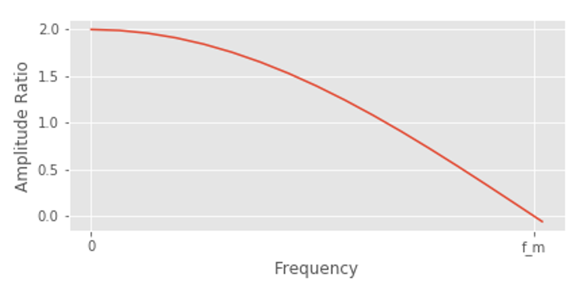
The following chart shows the magnitude response of a filter with the difference equation: $x[n] + x[n - 1]$.

Here is the code to implement a one sample delay filter in SuperCollider.

SynthDef(\oneSampleDelay, {
    arg out = 0, in;
    var sig = In.ar(in, 1);
    sig = sig + Delay1.ar(sig);
    Out.ar(out, sig);
}).add;

One-sample delays make poor filters but are simple to implement and understand.