CS112: MAT Files and Subplots
Storing and retrieving variables in MAT files
The names and values of variables generated in MATLAB can be stored in files for later use.
A special type of file called a MAT-file stores this information in a format that only MATLAB
understands. (Later we'll learn about how to work with files that can be read with a text
editor, Excel, and other application programs.) A MAT-file has a name with .mat
as the file extension, such as depthData.mat. The save command
stores variables in a .mat file. It can be called in several ways, as shown in
the following examples:
% create two variables to save
times = [0 1 2 3.5 7];
temps = [93.5 90.6 87.7 83.9 76.6];
% save times and temps in a file named data.mat using "command" format
save data.mat times temps
% save can also be called using "function" format
save('data.mat', 'times', 'temps')
% MATLAB creates a .mat file by default if this extension is omitted
save data times temps
% only save the temps variable
save data.mat temps
If a file already exists with the specified name, it is replaced by a new version of this
file. Unless otherwise specified, the new file is placed in the Current Directory. Other variables
may exist in the MATLAB Workspace, but only those specified in the call to save are
stored in the file.
The load command is used to retrieve variables from .mat files, and
can also be called in a variety of ways. For the following examples, assume that both
times and temps have been stored in data.mat.
% load the variables named times and temps into the MATLAB Workspace
load data.mat times temps               % command format
load('data.mat', 'times', 'temps');     % function format
% load a subset of the variables stored in the file
load data.mat temps
% both the .mat file extension and variable names are optional - in
% the following example, all variables stored in data.mat are loaded
load data
The save and load functions can be called from a MATLAB program or
from the Command Window. We will use the command format for calling these functions, but you
may see the function format in other MATLAB code that you read.
Displaying multiple plots
We have seen that the figure command can be used to display multiple plots in separate
figure windows. Multiple plots can be displayed within a single figure window using the
subplot function, which can be called as follows:
subplot(rows, cols, whichArea)
A (rows x cols) grid of plotting areas is created inside one figure window, with
each plotting area having its own axes. The whichArea input specifies which plotting
area to use for the next call to the plot function. The number 1 refers to the upper
left area, and the numbers increase from left to right across each row, and increase from the top to
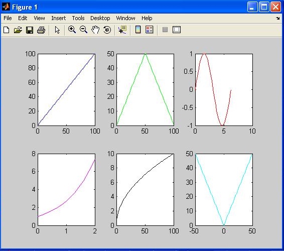
bottom rows, similar to the numbers of the days on a calendar. In the following code example,
a grid of plotting areas with 2 rows and 3 columns is created, and a different function is plotted
in each area, as shown in the picture below the code. The subplot function is called
before each call to plot, to specify where to display each graph.
Note that in each call to the plot function, the x and y coordinates are
created using colon notation that is provided as direct input to plot. It is
not necessary to place these coordinates in separate vectors that are created with an
assignment statement and supplied, by name, to the plot function.
figure
subplot(2, 3, 1)
plot(1:100, 'b')                    % single blue line
subplot(2, 3, 2)
plot(1:100, [1:50 50:-1:1], 'g')    % two green lines
subplot(2, 3, 3)
plot(0:pi/20:2*pi, sin(0:pi/20:2*pi), 'r')   % red sinusoid
subplot(2, 3, 4)
plot(0:0.1:2, exp(0:0.1:2), 'm')    % magenta exponential function
subplot(2, 3, 5)
plot(1:100, sqrt(1:100), 'k')       % black square-root function
subplot(2, 3, 6)
plot(-50:50, abs(-50:50), 'c')      % two cyan lines
