CS 112 Assignment 3

Due: Friday, February 27

You can turn in your assignment up until 5:00pm on 2/27/15. You should hand in both a hardcopy and electronic copy of your solutions. Your hardcopy submission should include printouts of four code files: illusion.m, grades.m, energy.m, and recognize.m. To save paper, you can cut and paste all of your code files into one script, but your electronic submission should contain the separate files. Your electronic submission is described in the section Uploading your completed work.

Reading

The following material from the fourth or fifth edition of the text is especially useful to review for this assignment: pages 39-53, 63-68, 72-78. You should also review notes and examples from Lab #4 and Lecture #7 (material on matrices, which may be continued on the day of Lecture #8).

Getting Started: Download assign3_programs from cs112d

Use Fetch or WinSCP to connect to the CS server using the cs112d account and download the assign3_exercises folder from the cs112d directory onto your Desktop. This folder contains two code files and three image files for Lab #4 and the exercises in this assignment.

Uploading your completed work

When you have completed all of the work for this assignment, your assign3_exercises folder should include two code files for the exercises, illusion.m and grades.m. Your assign3_problems folder should contain two code files named energy.m and recognize.m. Use Fetch or WinSCP to connect to your personal account on the CS file server and navigate to your cs112/drop/assign3 folder. Drag your assign3_exercises and assign3_problems folders to this drop folder. More details about this process can be found on the webpage on Managing Assignment Work.

Exercise 1: The Thatcher Illusion

The so-called Thatcher illusion was first demonstrated by the psychologist Peter Thompson in 1980. Follow this link to a fun page that allows you to experience the illusion yourself. The photographs of people on this page have been altered so that their eyes and mouth are flipped upside-down. When you view the altered images upside-down, you hardly notice, but when you flip the images upright, the result can look like something out of a horror movie! You can read more about the Thatcher illusion, or Thatcher effect, at this Wikipedia page. In this exercise, you'll create your own demonstration of this effect.

To begin, run the script named loadImages.m in the assign3_exercises folder, which loads two images that are assigned to the variables ellen and clinton in the MATLAB Workspace. For your demonstration, you can just choose one of these images, and you only need to flip the eyes upside-down. View your selected image with imtool and determine the coordinates for the corners of a rectangular region containing the eyes.

Create a script named illusion.m in the assign3_exercises folder, and add code to this script to create and display images that capture this illusion. In particular, your code should use subplot to create a 2 x 2 grid of four images, displayed as described below:

1. The original upright face image, with normal, upright eyes
2. The original image (from #1), viewed upside-down
3. A new image with the face shown upright and the eyes upside-down
4. The new image viewed upside-down (i.e. the face appears upside-down and the eyes appear upright)

It does not matter where you place the four images within the subplot. The Wikipedia page shows a sample display that is similar to what you should create for this problem. Tip: create a new variable to store the modified image that has the eyes upside-down.

Add comments to your illusion.m code file, with the names of you and your partner, the date, and a description of the task coded, and upload it with the other files in your assign3_exercises folder, when turning in Assignment 3.

Exercise 2: Working with gradesheets

The following table provides the semester grades for six CS112 students:

Name Homework Partic. Exam 1 Exam 2 Final Project Ann 83 90 76 80 88 Barb 79 80 80 81 70 Chelsea 90 90 92 98 94 Diana 72 75 63 75 73 Ella 88 90 78 89 82 Fiona 67 65 69 72 80

Open the file called grades.m in the assign3_exercises folder. This file creates a matrix named scores that contains the information in the above table, and two cell arrays called names and measures that store the names of the students and the components of the grade. Add code to the grades.m code file to perform the tasks listed below. Try to write code that is as compact as possible but still readable and understandable.

• Plot the Exam 1 and Exam 2 scores for the six students on a single graph, with the y-axis ranging from 50 to 100.
• Add a new column to the scores matrix with each student's final course score. The course score is calculated in CS112 as follows: Homework counts 40%, Participation 5%, Exams are each 20% and the Final Project is 15%.
• Create a new vector avgScores with the average (across students) of each component of the final grade, as well as the average final course grade.
• Print the names of the students whose final course score is higher than the class average.
• Print the names of the grade components that received the highest and lowest average scores.
• Plot the final course grades for the six students on the same graph as the Exam 1 and 2 scores, and add a horizontal line across the graph whose height is the average final course grade (for reference).
• Add a title, axis labels and legend to the graph.

Add comments to your grades.m file describing each of the above tasks, and also add comments with the names of you and your partner.

Problem 1: Energy production and consumption

In this problem, you will explore data on U.S. energy production and consumption using energy statistics available from the Energy Information Administration (EIA) within the U.S. Department of Energy. The assign3_problems folder in the course download directory contains two Excel spreadsheets, production.xls and consumption.xls, that were downloaded from the Energy Overview page at the EIA website. These spreadsheets contain both numerical and textual data related to the production and consumption of various energy sources over the years 1949-2006, which you can view by opening these files in Excel. Unfortunately, a separate MATLAB toolbox is needed to load data from complex spreadsheets such as this, and the public computers at Wellesley do not currently have this toolbox. We can, however, read Excel spreadsheets that contain only numerical data into MATLAB. The two files, produce.xls and consume.xls, contain most of the numerical data from the original EIA spreadsheets. These files can be read into MATLAB using the xlsread function, for example:

productionData = xlsread('produce.xls');

The contents of both produce.xls and consume.xls will be loaded into matrices with 58 rows corresponding to the years 1949-2006. The matrix created from produce.xls has 14 columns representing (1) year, (2) coal, (3) natural gas, (4) oil, (5) NGPL (natural gas plant liquids), (6) total fossil fuels, (7) nuclear, (8) hydroelectric, (9) geothermal, (10) solar, (11) wind, (12) biomass, (13) total renewable energy and (14) total energy produced. The matrix created from consume.xls contains 13 columns representing (1) year, (2) coal, (3) natural gas, (4) oil, (5) total fossil fuels, (6) nuclear, (7) hydroelectric, (8) geothermal, (9) solar, (10) wind, (11) biomass, (12) total renewable energy and (13) total energy consumed. The file population.mat in the assign3_programs contains a column vector of the U.S. population over the years 1949-2006.

Create a script file named energy.m in the assign3_problems folder that reads in the contents of the produce.xls, consume.xls and population.mat files and performs the following tasks:

Task 1: Plot the raw data

In a single figure window, plot the following data in one graph: amount of coal, gas, oil, NGLP, nuclear and total renewable energy produced, and the amount of coal, gas and oil consumed (note that the U.S. consumes all of the renewable energy sources that it produces). Plot this data as a function of the year. There should be 9 line plots drawn in a single plotting area. Complete this code without creating any additional variables - each call to the plot function should refer directly to the two matrices storing the data. Use one line style for all of the production data and a different line style for all of the consumption data, and use different colors for the plots. Add a title, axis labels and legend for the graph. Note that you can drag the corners of the figure window to expand its size, and drag the legend to a new location if desired.

Task 2: Graphical analyses of the data

Open a second figure window and create four graphs that display the following information for each year. In each case, the year can be plotted on the x axis. Use subplot to define a 2 x 2 grid of plotting areas for drawing the four graphs.

1. the fraction of total energy consumed that is produced in the U.S.
2. the amount of foreign oil that was needed to support the demand (i.e. the difference between oil consumed and produced)
3. the percentage of energy consumed that comes from renewable sources
4. the per capita total consumption of all energy sources combined

These observations are unfortunately a little disturbing...

Add comments to your energy.m code file.

Problem 2: Recognizing famous Wellesley alums

Wellesley College is proud to have some very distinguished alumnae! For this problem, you'll write a program to recognize the faces of three of our special graduates: Madeleine Albright '59, Hillary Clinton '69 and Pamela Melroy '83. The assign3_problems folder contains three face images whose identity is assumed to be known (albright.jpg, clinton.jpg, melroy.jpg) and three face images to be recognized by your program (face1.jpg, face2.jpg, face3.jpg). The file recognize.m contains initial code that loads the six face images into variables in the MATLAB workspace and displays them using subplot and imshow (the top three images are the known faces and the bottom images are the "unknown" faces):

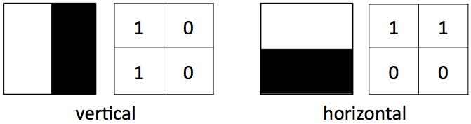
One strategy we can use to recognize an unknown image is to measure the difference between the pattern of brightness values in the unknown image and the patterns of brightness in each of a set of known images. We can then select the known image that represents the closest match. Consider a very simple example where we have two known image patterns corresponding to a vertical or horizontal edge, as shown below:

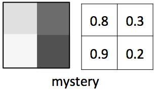
Suppose we are given a "mystery" image and want to determine whether it has a vertical or horizontal edge pattern:

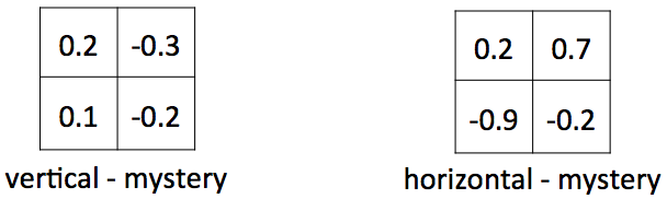
We can first calculate the element-by-element difference between each known image and our new mystery image:

We are really only interested in the amount of difference between the two patterns, so we can take the absolute value of the differences (this can be done with the abs function in MATLAB):

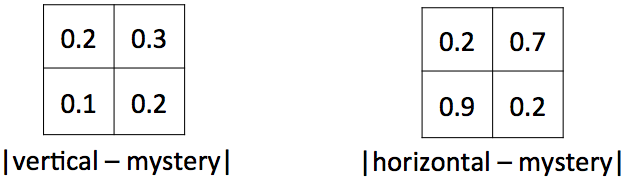
On average, the brightness values in the mystery image differ from the brightness values in the vertical image by only 0.2, while the brightness values differ from those in the horizontal image by 0.5 (on average). Thus there is a closer match between our mystery image and the vertical image, so we recognize it as a vertical edge.

Recognition using the full face images

Using this strategy for calculating how well the pattern of brightnesses match between two images, first add code to the recognize.m code file to calculate the average difference between the face1 image and each of the three known face images stored in the variables albright, clinton and melroy. Then add code to determine which of the three known faces is the best match to face1 using the three average differences that you calculated. Print a message indicating the identity of face1. Then repeat this process for the unknown faces stored in face2 and face3. Tip: cutting and pasting, and then making small modifications to the copied code, will save a lot of time! Your program should be able to recognize each of the three faces correctly.

Recognition using partial images

Real face recognition systems face many challenges: hair styles change and faces appear with different expressions, poses and directions of gaze, and with different backgrounds and lighting. To cope with variations in hair styles and backgrounds, the recognition process is often based on a cropped area of the face that excludes the hair and background. For this part of the problem, you'll attempt to recognize the three faces using a cropped region of the faces that includes only the eyes, nose and mouth. The original images (the images in the top row of Figure 1 above, labeled with each person's name) were carefully constructed so that they have the same overall size, with the region around the eyes, nose and mouth covering roughly the same area of each image. Create a set of six new variables that each store a small region of one of the original face images containing only the eyes, nose and mouth. Use the same coordinates for the upper left and lower right corners of the rectangular region that you select for all six images. Use imtool to help identify appropriate coordinates (as you move your mouse over the image displayed with imtool, the (X,Y) coordinates of the mouse are displayed in the lower left corner of the display window - remember that the order of these coordinates should be reversed when specifying the row and column of the corresponding locations of the matrix storing the image). Using subplot and imshow, display the six cropped images, as shown in the example below (again consider copying, pasting and modifying code here!):

Repeat your code to recognize the cropped versions of the face1, face2 and face3 images. Tip: copy and paste the code that you created to recognize the full images, and then make modifications to this code to use the cropped images instead. Are you still able to recognize each of the three faces correctly?

Note: you may have found the code in this problem to be very repetitious! This provides good motivation for learning our next topics: user-defined functions and loops.

Be sure to add comments to your recognize.m code file, describing the code. Also add comments at the top of the file indicating your name and that of a partner, and any collaborators.