CS 112 Assignment 8

Due: Thursday, May 6

You can turn in this assignment up until the last day of final exams, Monday, May 17, without penalty. Your hardcopy submission should include a cover sheet and a printout of the following code files: mobius.m, findStars.m, mapGUI.m and snowflake.m. Your electronic submission is described in the section Uploading your saved work

Reading

Getting Started: Download assign8_programs from cs112d

Uploading your saved work

• Browse through your directory and find the drop/assign8 folder
• Upload your assign8_programs folder into your drop/assign8 folder
• When done uploading, be sure to delete your assign8_programs folder from the Desktop by dragging it to the trash can, and then empty the trash (Finder--> Empty Trash).
• Be sure to Exit out of MATLAB when you are done

When you are done with this assignment, you should have ** files stored in your assign8_programs folder: mobius.m, milkyWay.jpg, findStars.m, mapGUI.fig, mapGUI.m, places.m, snowflake.m and drawOneStar.m.

Problem 1: Creating a Mobius Strip

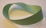
The Mobius strip was discovered in 1858 by the German mathematician August Mobius. Here's the easiest way to make one: take a strip of paper and instead of taping it together to make a link, twist one end and then tape the edges together. Now you have a Mobius strip. As a result of the half twist, the Mobius strip has only one side and one edge. If you draw a line down the middle of the strip until you get back to your starting point, you will draw on both sides of the paper. We'll use MATLAB to visualize a Mobius strip in 3D.

A Mobius strip can be represented with the following parameterized equations:

  x(u,v) = cos(u) + (v/2)*cos(u/2)*cos(u)
  y(u,v) = sin(u) + (v/2)*cos(u/2)*sin(u)
  z(u,v) = (v/2)*sin(u/2)

where 0<=u<=2π and -1<=v<=1. These equations create a Mobius strip of width 1 whose center circle has radius 1 and is centered at (0, 0, 0). The parameter u runs around the strip while v moves from one edge to the other. Here is a sample Mobius strip in MATLAB:

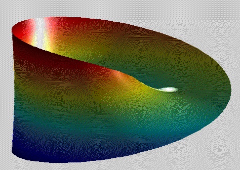
Write a function called mobius that creates a mobius strip as described above. You can display your strip as you like, the one shown above is just an example. Your function set the view, colormap, lighting, material property and shading of your mobius strip. Write brief comments providing usage information for your function, so that typing help mobius in the Command Window prints a short function description.

Problem 2: Reaching for the Stars

Your goal for this problem is to count the stars in NASA's Astronomy Picture of the Day from October 23, 2005. The milkyWay.jpg file in the assign8_programs folder contains this NASA image, which can be loaded into the MATLAB Workspace using imread. The image is automatically loaded in as a 516x624x3 matrix of type uint8. The third dimension stores red, green and blue (RGB) color components as integers ranging from 0 to 255. This color image can be displayed with imshow.

The stars in the MilkyWay image are bright white areas. Recall that in the RGB color representation, white is composed of maximum values of all three RGB colors. You can find the stars in the image by first finding locations with large red, green and blue values (i.e. locations that are close to white), and then counting the clusters of white locations. You will write a function that uses this strategy to count the stars, and also displays intermediate results along the way.

More specifically, write a function findStars that has two inputs, an image and a threshold, and performs the steps listed below:

1. In one figure window, use subplot to create a 2x2 configuration of four images: the original image, and three gray-level images that depict the red, green and blue components of the original image (similar to our Mona Lisa example in lecture).
2. Find the stars: create a 2-D matrix of logical values that is the same size as the input image. In this matrix, store a 1 at locations where the red, green and blue values in the input image are all above the input threshold
3. Count the stars: use bwlabel to find the connected components of the logical matrix that you created. Connected components are groups of 1's that are connected in the image (the second input to bwlabel can be 4 or 8, depending on whether you want to consider diagonal elements as connected). The groups of image locations that are connected are all labeled with the same number, and the label number increases with each new connected component that is found. Determine the number of stars found (the number of connected components, which will be the largest number stored in the matrix of component labels).
4. Display the stars with your own colormap: create your own colormap to display the connected components corresponding to stars - the number of colors should equal the number of stars, so that each label is displayed with a different color. For example, you could just create multiple shades of your favorite color. The index 1 in the colormap should store the color black, and colors for labels should be sufficiently large RGB values to be visible. In a separate figure window, display the star components using your colormap - imshow can display an indexed image where each value is an index into a colormap: imshow(components, colormap).
5. Finally, print a message in the Command Window that indicates how many stars were found.

Problem 3: Wellesley Campus Places

In this problem, you'll create a simple GUI to display the locations of popular campus places on an aerial view of campus:

The assign8_programs folder contains an aerial image of the Wellesley campus, in wellesley.bmp, and a file places.m that contains a function that creates and returns a cell array of the names of some public places on campus and a 14x2 matrix with the (x,y) coordinates for these places. Use guide to create a GUI that includes a display area, listbox, label and close button. Your program can call the places function to create the cell array of names and matrix of coordinates, and then load the list of campus names into the listbox by setting the String property for the listbox component to the cell array of names. After the aerial image is displayed on the GUI, the scatter function can be used to draw a marker (a star in the above picture) at a particular location on the map. When the user selects a new place in the listbox, the marker should move to the newly selected campus location.

Problem 4: Koch Snowflakes

snowflake(0,0,1,200,'b');	snowflake(0,0,2,200,'b');
snowflake(0,0,3,200,'b');	snowflake(0,0,4,200,'b');
snowflake(0,0,5,200,'b');

Let's take a close look at the level 2 figure to understand how the Koch snowflake is drawn:

snowflake(0, 0, 2, 200,'b')

snowflake(xcenter, ycenter, level, sideLength, color)

The left side above shows the Koch snowflake at level 2 in blue. The lower left hand corner of the snowflake is at position (0,0). Each side of the biggest triangle has length 200. The right side shows the six pink stars (each pink star is made of triangles with length 200/3) that are overlaid on top of the original star to produce the level 2 image (as an aside, note the cool snowflake pattern in the middle). Note the blue circles at the lower left corner of each of the six stars. Think of these as the anchors for each of the smaller stars.

We need to know the coordinates of all six anchor points in order to be able to draw the Koch snowflake. We are given the coordinates of only one point, the lower left corner marked as (x,y). In this particular image, x and y are both 0. The left image shows grid lines connecting the six blue anchor points. The right image illustrates that if we can calculate xoffset and yoffset, then we can figure out the x and y coordinates of all six anchor points of our pink stars. The blue line marked side is the length of the original star. You can see from the diagram that the xoffset is one-third the length of the side.

The yoffset, however, requires a bit of geometry. We use the Pythagorean theorem to derive the length of yoffset, since we know the length of two sides of a right triangle. The yoffset, then, is the square root of the difference of the squares of the two lengths (side/9 and 2*side/9) shown in the diagram above.

Given the grid above and the xoffset and yoffset distances, now all the anchor coordinates of the six star positions are calculated. In the assign8_programs folder, you will find drawOneStar(x,y,sideLength,color) which creates the six-pointed star shown here.

drawOneStar(0,0,100,'m')

Note that the image produced by drawOneStar matches the image drawn by snowflake at recursion level 1 (shown above).

Hints:

• Look at the images above and try to figure out how a figure at one level is created, and how it uses figures from the previous level.
• It's easiest to display recursive figures by doing something like this:

  >> figure
>> hold on
>> snowflake(0,0,2,200,'b');
>> hold off


  The hold on is critical, otherwise you will only see the most recent plot, rather than all the plots at the different levels combined.

• Test up to, but not greater than, recursion level 5. A recursion level higher than 5 is likely to take a long time (> 20 minutes).