Assignment 8
![]()
|
|
CS 112
Assignment 8
|
|
You can turn in your assignment up until 5:00pm on 5/2/08 without
penalty, but it is best to hand in the assignment at the beginning of
class. Your hardcopy submission should include a cover sheet and a printout of the following code files:
mobius.m, birdDB.m, findStars.m, and snowflake.m. Your electronic
submission is described in the section Uploading your saved work
assign8_programs folder from the cs112d directory
onto your Desktop. Rename the folder to be yours, e.g. sohie_assign8_programs.
In MATLAB, set the Current Directory to your assign8_programs folder.
drop/assign8 folder
assign8_programs folder into your
drop/assign8 folder
assign8_programs folder from the Desktop by dragging
it to the trash can, and then empty the trash (Finder--> Empty Trash).
When you are done with this assignment, you should have 8 files
stored in your assign8_programs folder: mobius.m, birds.txt, birdDB.m,
milkyWay.jpg, findStars.m, snowflake.m, drawOneStar.m and findStars.m.
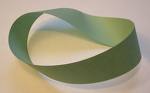
The Mobius strip was discovered in 1858 by the German mathematician August Mobius. Here's the easiest way to make one: take a strip of paper and instead of taping it together to make a link, twist one end and then tape the edges together. Now you have a Mobius strip. As a result of the half twist, the Mobius strip has only one side and one edge. If you draw a line down the middle of the strip until you get back to your starting point, you will draw on both sides of the paper. We're going to use MATLAB to visualize a Mobius strip in 3D.
A Mobius strip can be represented with the following parameterized equations:
x(u,v) = cos(u) + (v/2)*cos(u/2)*cos(u)
y(u,v) = sin(u) + (v/2)*cos(u/2)*sin(u)
z(u,v) = (v/2)*sin(u/2)
where 0<=u<=2π and -1<=v<=1. These equations create a Mobius strip of width 1 whose center circle has radius 1 and is centered at (0, 0, 0). The parameter u runs around the strip while v moves from one edge to the other. Here is a sample Mobius strip in MATLAB:
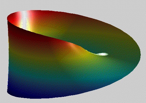
Write a function called mobius.m that creates a mobius strip as described above. You can display your strip as you like, the one shown above is just an example.
Your function must include setting the view, colormap, lighting and shading
of your mobius strip. You can also explore reflectance properties of surfaces using the material function in MATLAB. Remember to write brief comments providing usage information
for your function (e.g. so that if one types help mobius in the command window, a terse function description would appear).
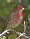
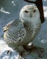
In lecture, we worked with a database of information about many species
of birds that inhabit the New England area. This problem builds on that work, to
explore the bird species further and generalize the functions for selecting and sorting
the bird information. The code presented in lecture is contained in the birdDB.m
file in the assign8_programs folder. The birds.txt file contains
information about 60 species of birds,
including their name, family, habitat, size, wingspan, dominant color(s) of the back, underside
and head of the species, whether or not the bird has spots, and a comment about a
salient feature of the species. For simplicity,
each value is stored as a string of contiguous non-space characters, with capitalization or
punctuation (/) used to separate multiple words.
The birdDB.m file contains a top-level function at the beginning named
birdDB that has no inputs or outputs. This function loads the birds.txt
text file into a large
cell array named birds and prints the contents of birds with the
printBirdInfo function defined in this file. The rest of the
birdDB function contains code for testing the following additional functions
defined in this file: getBirds, getHerons, getWetlands, getBigWings,
sortByName and sortByWingspan. Add code to the birdDB.m file to
complete the following tasks:
The getHerons, getWetlands and getBigWings functions each return
a vector of indices of birds in the birds cell array that satisfy a single criterion.
The function handle for each of these functions, designated by the @
character before the function name, can be supplied as an input to the general
getBirds function that returns a new cell array containing only those birds satisfying
the desired criterion. The top-level birdDB function contains code illustrating
the application of these functions. Define a new criterion function that is similar to the
getWetlands function, which returns the indices of sandpipers whose size is larger
than 10 inches and who inhabit mudflats. Add code to the birdDB function to test your
new function.
The sortByName and sortByWingspan functions contain substantial code
that is the same as code in the getBirds function. In fact, the getBirds
function
itself can be used for sorting. In this case, the input criterion function should return
a vector of indices that can be used to rearrange the contents of the birds cell array
in sorted
order. Define two criterion functions sortNames and sortWings that
can be supplied as an input to getBirds to create a new cell array of bird
information in which the birds are sorted by name or wingspan (these two functions will be short,
similar to getHerons and getBigWings). Again add code to the
birdDB function to test your new functions.
Write a function named printNames that has a single input cell array that
is assumed to have the structure of the birds cell array, which prints only the
names of all of the bird species contained in the input cell array. Add code to the
birdDB function to test printNames.
At this point, you have lots of short, specialized criterion functions for selecting and sorting
the bird species, which can be supplied as an input to the getBirds function,
for example:
>> wetlands = getBirds(birds, @getWetlands)
The getWetlands function returns the indices of birds that have a string
in the third cell of the birds cell array that contains the substring
'wetlands'. It would be nice to have a more general criterion
function that returns the indices of birds from any cell of the birds cell array
that has a string containing any substring of interest.
Similarly, the sortNames and sortWings functions that you wrote for part (2)
return a vector of indices that can be used to sort the contents of particular cells
of the birds cell array. It would be nice to have a more general criterion
function that returns a vector of indices that can be used to rearrange the contents of
any cell of the birds cell array in sorted order. Add code to allow these
generalizations. In particular:
getBirdsAny that has three inputs: the birds
cell array, an index of the birds cell array, and a string. This function should
return the indices of birds that have a string in the requested cell that contains the
input string. For example, the following function call:
indices = getBirdsAny(birds, 8, 'brown')
should return a vector of indices of all birds that have the string 'brown' in their
head color (in some cases, it may be a substring, e.g. 'brown/white').
sortAny that has two inputs: the birds cell array
and an index for this cell array. This function should return a vector of indices that can
be used to sort the contents of the requested cell of the birds cell array. For example,
the following function calls:
 indices = sortAny(5);

indices = sortAny(1);
should return vectors of indices that can be used to sort the birds by increasing wingspan and
alphabetically by name, respectively. The function iscell can be used to determine
whether a particular cell of the birds cell array contains a cell array (of strings)
or a vector (of numbers) inside.
getBirds function to have two additional optional inputs
corresponding to an index of the birds cell array and a string. If getBirds
is called with three inputs (birds, a criterion function such as
@sortAny and an index), then the criterion function should be called with the
index as an additional input. If getBirds is called with four inputs
(birds, a criterion function such as @getBirdsAny, an index and a string),
then the criterion function should be called with the index and string as additional inputs.
birdDB function to test your new functions.
Your goal for this problem is
to count the stars in NASA's
Astronomy Picture of the Day from October 23, 2005. The milkyWay.jpg
file in the assign8_programs folder contains this NASA image, which can be
loaded into the MATLAB Workspace using imread. The image is automatically loaded
in as a 516x624x3 matrix of type uint8. The third dimension stores red, green and blue
(RGB) color components as integers ranging from 0 to 255. This color image can be displayed with
imshow.
The stars in the MilkyWay
image are bright white areas. Recall that in the RGB color
representation, white is composed of maximum values of all three RGB colors. You can find the
stars in the image by first finding locations with large red, green and blue values (i.e.
locations that are close to white), and then counting the clusters of white locations. You will
write a function that uses this strategy to count the stars, and also displays
intermediate results along the way.
More specifically, write a function findStars that has two inputs, an image
and a threshold, and performs the steps listed below. All of the display steps can be
performed with the imshow function, and will be displaying images in three
separate figure windows. Recall that the figure command opens a new
figure window. After running the findStars function, execute the close all
command to close the existing windows before running findStars again. MATLAB behaves in
a buggy manner when too many large figure windows are open at one time.
findStars function to perform the following steps:
subplot to create a 2x2 configuration of four
images: the original image, and three gray-level images that depict the red, green and blue
components of the original image (similar to our Mona Lisa example in lecture).
size function returns a vector with all three
dimensions in the case of a 3-D matrix, and an initial matrix of the logical value
0 can be created with the false function, e.g.
matrix = false(10,10,3)).
(x,y,1) is greater than the input threshold, then store a 1 at
location (x,y,1) in the 3-D logical matrix. (When calling
findStars, keep in mind that the RGB values range from 0 to 255, so choose
a threshold in this range.)
subplot to create a new 2x2 configuration
of four images: the red, green and blue slices of the 3-D logical matrix created in
step 2b, and the 2-D matrix created in step 2c.
bwlabel to find the connected components of the binary
image (logical matrix) that you created in step 2c. Connected components are groups of
1's that are connected in the image (the second input to bwlabel can be
4 or 8, depending on whether you want to consider diagonal elements as connected). The
groups of image locations that are connected are all labeled with the same number, and
the label number increases with each new connected component that is found.
imshow can display an indexed image where each value is an index
into a colormap: imshow(components, colormap).
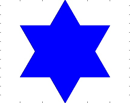
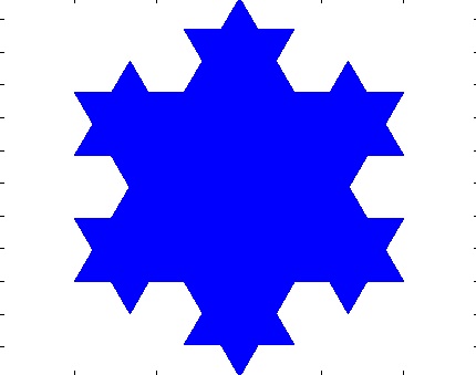
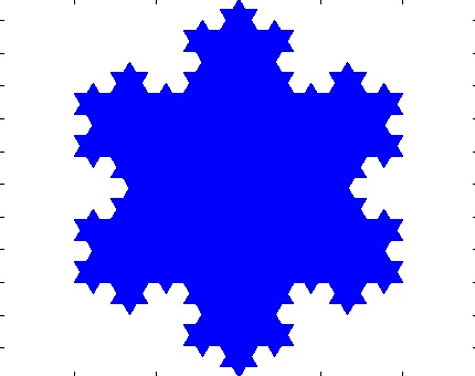
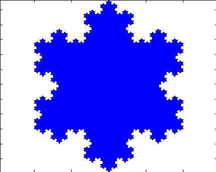
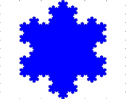
snowflake.m that produces the pictures below. The
function snowflake takes 5 inputs: xcenter, ycenter,
levels, sideLength and color.
snowflake(0,0,1,200,'b'); |
snowflake(0,0,2,200,'b'); |
|
|
snowflake(0,0,3,200,'b'); |
snowflake(0,0,4,200,'b'); |
|
|
snowflake(0,0,5,200,'b'); |
|
|
Let's take a close look at the level 2 figure to understand how the Koch snowflake is drawn:
snowflake(xcenter, ycenter, level, sideLength, color) | |
|
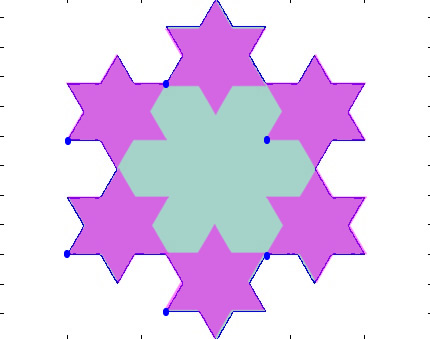 |
The left side above shows the Koch snowflake at level 2 in blue. The lower left hand corner of the snowflake is at position (0,0). Each side of the biggest triangle has length 200. The right side shows the six pink stars (each pink star is made of triangles with length 200/3) that are overlaid on top of the original star to produce the level 2 image (as an aside, note the cool snowflake pattern in the middle). Note the blue circles at the lower left corner of each of the six stars. Think of these as the anchors for each of the smaller stars.
 | 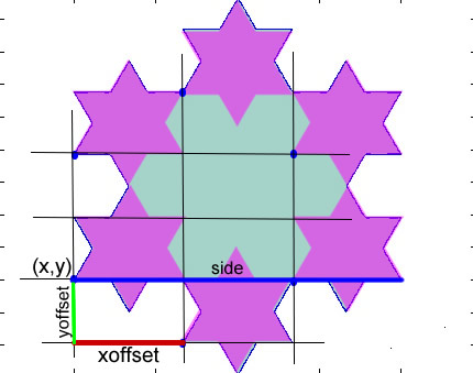 |
We need to know the coordinates of all six anchor points in order to
be able to draw the Koch snowflake.
We are given the coordinates of only one point, the lower left
corner marked as (x,y). In this particular image, x and y are both 0.
The left image shows grid lines connecting the six blue anchor points.
The right images illustrates that if we can calculate xoffset
and yoffset, then we can figure out the x and y coordinates of
all six anchor points of our pink stars. The blue line marked side
is the length of the original star.
You can see from the diagram that the xoffset is one-third the length of the side.
 |
The yoffset, however, requires a bit of geometry. We use the Pythagorean theorem to derive the length of yoffset, since we know the length of two sides of a right triangle. The yoffset, then, is the square root of the difference of the squares of the two lengths (side/9 and 2*side/9) shown in the diagram above.
Given the grid above and the xoffset and yoffset distances, now all the anchor coordinates of the six star positions are calculated.
In the assign8_folder, you will find drawOneStar(x,y,sideLength,color) which creates the six-pointed star shown here.
drawOneStar(0,0,100,'m') | |
 |
Note that the image produced by drawOneStar matches the image drawn by snowflake at recursion level 1 (shown above).
Hints:
>> figure

>> hold on

>> snowflake(0,0,2,200,'b');

>> hold off
The hold on is critical, otherwise you will only see the most recent plot, rather than all the plots at the different levels combined.