Computation for the Sciences Assignment 2

Computation for the Sciences

Assignment 2

Due Date: TBA

Your hardcopy submission should include printouts of 4 code files: lab3.m, redsox.m, colonTest.m, analyzeData.m.

Reading

The following material in the text is useful to review for this assignment: pages 53-58, 65-72. You should also review notes and examples from Lectures #4 and #5, and Lab #3.

Getting Started: Download assign2_programs from the download directory

Download a copy of the assign2_programs folder from the download directory onto your Desktop. Rename the folder to be yours, e.g. stella_assign2_programs. In MATLAB, set the Current Directory to be your renamed assign2_programs folder on your Desktop.

When you are done with this assignment, you should have 4 code files stored in your assign2_programs folder: lab3.m, redsox.m, colonTest.m, analyzeData.m.

Exercise 1: Practice with conditional expressions

Create a new file in MATLAB called lab3.m (that you will turn in). Make sure your current directory is set appropriately.

In lab3.m, first use MATLAB's input function to prompt the user for three pieces of information: 1) a numerical month (between 1 and 12), 2) a day (between 1 and 31) and 3) the user's name. Store each of these values in a variable (e.g. month is 7 (for July), day is 28 and name is 'Rosa'). To prompt the user for a string, provide a second input 's' when calling the input function:

name = input('Enter your name: ', 's'); % name is a string

Then write MATLAB expressions that correspond to the following:

Create a variable valentine that is true on February 14 and false otherwise.
Create a variable csMidterm that is true on March 9 and April 21 and false otherwise.
Create a variable springBreak that is true between March 23 and March 27 (inclusive).
Create a variable luckyDay that is true if the month and day are both odd or both even, and false otherwise.
If month and day are your birthday, then print out a personalized birthday greeting such as "Happy Birthday to Rosa!", otherwise print "Not Rosa's birthday". The disp function can be used to print text that combines literal strings with variables whose value is a string:
```
>> place = 'SCI 257';
>> disp(['class will be held in ' place ' today']);
class will be held in SCI 257 today
>>
```
If month is December, January or February, then print the lyrics of the first stanza of the song, "Let it Snow" (on four separate lines), otherwise print a message of your choosing (this can be a single line).

   Oh the weather outside is frightful,
   But the fire is so delightful,
   And since we've no place to go,
   Let it snow! Let it snow! Let it snow!

You can test your variables by inputting different values for month and day and then seeing if your variables contain the correct values. Add comments containing your name and date to your lab3.m file and upload it with your other MATLAB files in your assign2_programs folder, when turning in Assignment 2.

Exercise 2: The Red Sox roster

In this exercise, you'll work with the following subset of data from the Boston Red Sox baseball team roster from the 2007 (World Series winning!) season:

Player Name Player Number Weight At Bats Home Runs Batting Average 2007 Salary Runs Batted In Runs Stolen Bases

Jason Varitek 33 230 435 17 .255 11,000,000 68 57 1

David Ortiz 34 230 549 35 .332 13,250,000 117 116 3

Manny Ramirez 24 200 483 20 .296 17,016,381 88 84 0

J.D. Drew 7 200 466 11 .270 14,400,000 64 84 4

Mike Lowell 25 210 589 21 .324 9,000,000 120 79 3

Julio Lugo 23 175 570 8 .237 8,250,000 73 71 33

Kevin Youkilis 20 220 528 16 .288 424,500 83 85 4

Coco Crisp 10 180 526 6 .268 3,833,333 60 85 28

Dustin Pedroia 15 180 520 8 .317 380,000 50 86 7

Player Name	Player Number	Weight	At Bats	Home Runs	Batting Average	2007 Salary	Runs Batted In	Runs	Stolen Bases
Jason Varitek	33	230	435	17	.255	11,000,000	68	57	1
David Ortiz	34	230	549	35	.332	13,250,000	117	116	3
Manny Ramirez	24	200	483	20	.296	17,016,381	88	84	0
J.D. Drew	7	200	466	11	.270	14,400,000	64	84	4
Mike Lowell	25	210	589	21	.324	9,000,000	120	79	3
Julio Lugo	23	175	570	8	.237	8,250,000	73	71	33
Kevin Youkilis	20	220	528	16	.288	424,500	83	85	4
Coco Crisp	10	180	526	6	.268	3,833,333	60	85	28
Dustin Pedroia	15	180	520	8	.317	380,000	50	86	7

Generating some Red Sox statistics:

The file redsox.m creates 9 separate vectors for each numerical statistic. Look closely at the code in redsox.m and note that the names are stored in a cell array called names. Think of a cell array as a special kind of vector that allows us to store strings. Note that names is created using the curly brace { } rather than the square bracket [ ] that we use for numerical vectors. Although a cell array is created using the curly braces, you do not need to use curly braces to access its contents. For example, here is a clip of MATLAB code accessing the contents of names:

>> powerHitter = names(homeRuns > 20)
powerHitter =
     'Ortiz'   'Lowell'
>>

Note that you can place a semi-colon at the end of the initial assignment statements in redsox.m to suppress the printout of the statistics.

In the exercise below, you may use MATLAB's mean, sum, length, and any.

Write MATLAB code to do the following:

Create a variable totalStolen with the total number of stolen bases in 2007.
Create a variable avgWt with the average weight of a Red Sox player.
Create a variable bestBatters with the name(s) of player(s) whose batting average is greater than or equal to 0.300.
Create a variable expensiveHomer that is true if any player costs more than $500,000 per homerun.
Create a variable bigHitter that is true if any players hit more than 10 homeruns with batting averages less than .290.
Create a vector highRBI with the name(s) of player(s) whose Runs Batted In is greater than or equal to Runs.
Create a variable bigBatter that contains the number(s) of the player(s) with more than 550 at bats or more than 20 stolen bases.
Create a variable weightInGold that contains the number of players who are paid more than $25,000 per pound of body weight in the 2007 season.

Add comments to your code so that it is clear and easy to read. Always include your name and date at the top of each file. Save your final version of redsox.m in your assign2_programs folder to upload to the cs server.

Exercise 3: Indexing with colon notation

In lecture you learned how to use colon notation to specify a sequence of regularly spaced numbers. You also learned how to use indexing to read and store values in specific locations of a vector. This exercise combines these two concepts. Colon notation can be used to specify an evenly spaced sequence of vector indices or contents, as shown in the following examples:

>> nums = 1:8
nums = 
  1   2   3   4   5   6   7    8
>> nums(1:2:5) = 10
nums = 
  10   2   10    4   10   6   7   8
>> nums(2:3:8) = [13 9 16]
nums =
  10   13   10   4   9    6   7   16
>> nums2 = nums([1:3 6:8])
nums2 =
  10   13   10   6   7   16
>> nums([1:3 6:8]) = 12:-2:2
nums =
12   10   8   4   9   6   4   2
>>

The following program, colonTest.m is contained in your assign2_programs folder. Follow the instructions in the comments to rewrite the existing code statements and add five additional statements that use colon notation:

% colonTest.m
% program that provides practice with colon notation and indexing

% rewrite each of the next 4 statements using colon notation
nums1 = [10 9 8 7 6 5 4 3 2 1]
nums2 = nums1([2 4 6 8 10 7 4 1])
nums1([3 4 5 6]) = [9 6 3 0]
nums3 = [1 2 3 1 2 3 1 2 3]

% replace the next 3 statements with a single assignment statement
% that uses colon notation
nums2(6) = 10
nums2(7) = 20
nums2(8) = 30

% for each of the following examples, use "end" in the colon
% notation, for example: nums8 = nums1(3:end)

% write a statement that assigns nums4 to a vector that contains
% the odd-indexed elements of nums1

% write a statement that assigns nums5 to a vector of the
% elements contained in the top half (higher indices) of nums2

% write a statement that assigns nums6 to a vector that contains
% every 3rd element of nums1, starting with index 2

% write a statement that places the value 0 in all of the 
% evenly indexed locations of nums2

% write a statement that places the numbers 8 12 16 20 in the 
% successive odd-indexed elements of nums2

If you write each code statement with no semi-colon at the end, so that the value generated is printed out during execution of the code, then your program should generate the following printout:

>> colonTest
nums1 =
  10  9  8  7  6  5  4  3  2  1
nums2 =
   9  7  5  3  1  4  7  10
nums1 =
  10  9  9  6  3  0  4  3  2  1
nums3 =
   1  2  3  1  2  3  1  2  3
nums2 =
   9  7  5  3  1  10  20  30
nums4 =
  10  9  3  4  2
nums5 =
   1  10  20  30
nums6 =
   9  3  3
nums2 =
   9  0  5  0  1  0  20  0
nums2 =
   8  0  12  0  16  0  20  0
>>

Place comments at the top of your file with your name and date. Your final submission should include a copy of your final colonTest.m code file.

Problem: Cleaning up the data

Unreliable measurement instruments or unpredictable environments can sometimes yield data that is clearly erroneous. To obtain a reliable assessment of simple properties like the mean value of the data, it may be desirable to remove data samples that are clearly outside the expected range. Such samples are sometimes referred to as outliers. An advantage to analyzing data in MATLAB, with its general programming language, is that we can easily write a program to preprocess the data in a customized way. In this problem, you will complete a program that removes outlying data samples, using the mean and standard deviation of the data.

Imagine that you collected sonar data on the depth of the ocean floor over a large region that is essentially flat. Due to instrument problems and the occasional large marine animal, some measurements are clearly invalid. For simplicity, assume that all of the erroneous measurements are underestimates of the true depth of the ocean floor. The file analyzeData.m in your assign2_programs folder uses the load command to load 1000 depth measurements from a file named depthData.mat into a vector named depthData, and creates a plot of this initial data:

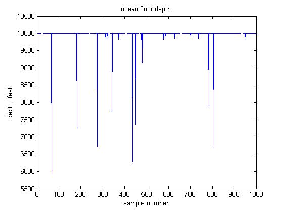
Most of the data is at a depth of around 10,000 feet. The erroneous data samples appear as downward spikes in the data, at depths that are significantly less than 10,000 feet. One principled way to go about removing outlying data is to remove samples whose value is far from the mean value, using the standard deviation to determine the range of values to remove. The standard deviation captures how spread out the data values are, and is given by the following formula:

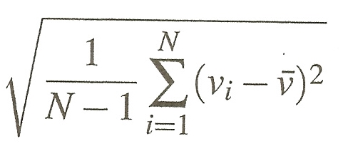
N is the number of samples in the data, v_i is the i^th data sample, and v is the mean value of the data. If the distribution of the data follows a bell-shaped curve (which is not really the case here), almost all of the data should lie within three standard deviations of the mean value (see here for more information).

For the ocean floor depth data, we could just remove all samples that are more than three standard deviations away from the mean depth value. A problem with this strategy is that an initial calculation of the mean and standard deviation of all of the data will be biased by the presence of the outlying data samples. Thus, we will instead use a more conservative approach that removes data in two stages, as described in the following steps, which also print, display and save the data:

calculate and print the mean and standard deviation of the original data
modify the data so that samples whose value is more than 4 standard deviations away from the mean value are removed
calculate and print the mean and standard deviation of the modified data, and plot the modified data
ask the user if she would like to remove more outliers from the data. If so,
- 4a. modify the data again so that samples whose value is more than 3 standard deviations away from the mean are removed, using the newly calculated mean and standard deviation from step 3
- 4b. calculate and print the mean and standard deviation of the newly modified data, and plot this new data
save the final modified data and its mean and standard deviation in a file named newData.mat

Expand the analyzeData.m code file to perform the above steps. When completing this program, keep in mind the following background, tips and guidelines:

The built-in mean function can be used to calculate the mean value of the data, but you must compute the standard deviation using the above formula. It is OK to use the built-in std function to check your calculation - you should obtain similar results. Keep in mind that the number of samples in the data changes after each modification.
Logical vectors can be used to represent the locations of values in a vector that satisfy a certain logical condition. Steps 2 and 4a describe which data values to remove - how can you rephrase these steps to describe which data values to preserve? This will facilitate your thinking about how to construct a logical vector that has a 1 in locations of data to preserve.
Create two variables to store the mean and standard deviation of the original data stored in the depthData vector, and re-use these two variable names to store the new mean and standard deviation in steps 3 and 4b. When modifying the data in steps 2 and 4a, re-use the same variable name, depthData.
Calculating the standard deviation and the modified data each involve multiple conceptual steps. Try to incorporate all of these steps into a single assignment statement for each of these two variables. Be careful about the placement of parentheses in these statements!
The values of variables can be printed by omitting the semi-colon at the end of assignment statements or by using disp. Remember that numbers need to be converted to strings when using disp:
```
>> slugs = 32.15;
>> disp(['there are ' num2str(slugs) ' slugs in a pound']);
there are 32.15 slugs in a pound
>>
```
When asking the user whether more outliers should be removed, assume that the user replies with a string, such as yes or no. Two strings can be compared with the strcmp function that returns true (logical value 1) if the two strings are equal:
```
name = input('Enter your name: ', 's');
if strcmp(name, 'Stella')
    disp('I know you! You''re our Lab Instructor!')
else
    disp('I don''t know you')
end
```
Click here for information about using .mat files to store and retrieve variables using save and load.
In Assignment 1, the figure command was used to display multiple plots in separate figure windows. Multiple plots can be displayed within a single figure window using the subplot function, described here. The analyzeData.m code file contains a call to subplot that specifies that the figure window should have one row of three plotting areas, and that the first plot should appear in the leftmost area. Use subplot to place the plot of the intermediate data in the center plotting area and the final data (if further analysis is requested by the user) in the rightmost area. You can expand the window in the horizontal direction by dragging the borders of the window horizontally. Note that the range of values plotted on the axes will differ for the three plots.
Place comments at the beginning of the code file with your name and date, and place a few comments throughout your program briefly describing what is accomplished by small groups of code statements.
At the end of your program, add comments that record the values of the mean and standard deviation after steps 1, 3, and 4b, and answer the following question: How did the mean and standard deviation change between the initial, intermediate and final data, and why did these quantities change in this way?

Your final submission should include a copy of your final analyzeData.m code file.