Assignment 4
![]()
|
|
Computation for the Sciences
Assignment 4
|
|
Your hardcopy submission
should include printouts of 5 code files: cs112_sat.m, ubbi.m, lineFit.m, poleVault.m
and virus.m.
assign4_programs folder from the download directory
onto your Desktop. Rename the folder to be yours, e.g. stella_assign4_programs.
In MATLAB, set the Current Directory to your assign4_programs folder.
When you are done with this assignment, you should have 6 code files, one .cfit file and one data
file stored in your assign4_programs folder: cs112_sat.m,
ubbi.m, lineFit.m, poleVault.m, virus.m, displayGrid.m, sat.cfit and
poleVaultdata.mat.

Write a function called ubbi that takes a string as input and
returns the ubbidubbified string as output. The rule for conversion is to
insert 'ub' in front of every vowel.
This clip of MATLAB's command window shows what the function ubbi
should do:
>>
>> newcs112 = ubbi('cs112')
newcs112 =
cs112
>>
>> test = ubbi('I am flying to America!')
test =
ubI ubam flubyubing tubo ubAmuberubicuba!
>>
Note in the examples above that
both lower case and upper case vowels work. You can put all the vowels into a single
string, which MATLAB will store in a vector of characters (see the colors
vector in the makeBullseye2 function in the Lecture #9 slides).
Recall that using square brackets allows for string concatenation, as in:
 >> disp(['a' 'whole' 'bunch'])

 awholebunch
The == operator can be used to compare a string with a single
character. In this case, it returns a logical vector that contains 1's at the locations
where the character appears in the string, for example:
>> 'banana' == 'a'

ans =

    0     1     0     1
    0     1
Your function ubbi should still work (i.e. no MATLAB error messages are
generated) if the user does not supply an input string, as shown in the example below:
>>
>> ubbi
Please supply a string to ubbidubbify
>>
>> ubbi('oooh, ok I will.')
ans =
uboubouboh, ubok ubI wubill.
>>
One true test of any scientific theory is whether or not it can be used to make accurate predictions. Given some data that captures the relationship between two or more variables, we can try to formulate a mathematical model that summarizes this relationship. If the model is valid, it can be used to predict the relationship between the variables in cases not explicitly given in the original data.
In some cases, variables may have a simple linear relationship, such as in
the forearm and hand data that we used to test the existence of the Golden Ratio:

The line drawn through the points is the best fit line for the data, also
referred to as the regression line. MATLAB provides functions for fitting lines
and other curves to data, but you'll instead write your own function to compute the
regression line for a set of data, and tailor the information that is returned.
You will then apply this analysis to data on the achievements
of olympic pole vaulters in the summer olympics, since they began in 1896. Finally, you
will analyze the pole vaulting data using the Curve Fitting Toolbox that you explored in
Exercise 1.
Computing a regression line
A nice introduction to the computation of regression lines is provided online at the Finite Mathematics & Applied Calculus Resource Page developed by Stefan Waner and Steven Costenoble at Hofstra University.
Given the (x,y) coordinates for a set of n points (x1,y1), (x2,y2), ... (xn,yn), the best fit line associated with these points has the form
y = mx + b
where
slope = m = (n(Σxy) - (Σx)(Σy)) / (n(Σx2) - (Σx)2)
intercept = b = (Σy - m(Σx)) / n
The Σ means "sum of", so
Σx = sum of x coordinates = x1 +
x2 + ... + xn
Σy = sum of y coordinates = y1 +
y2 + ... + yn
Σxy = sum of xy products = x1y1 +
x2y2 + ... + xnyn
Σx2 = sum of squares of x coordinates =
x12 + x22 + ... +
yn2
When performing linear regression, it is valuable to know how well the line actually
fits the data. Two measures used to assess the quality of fit are the correlation
coefficient and the size of the residuals that capture the difference between
the actual data values and the values predicted by the regression line. The correlation
coefficient, also described in the Waner and Costenoble online chapter, is a number
r between -1 and 1 calculated as follows:
coefficient = r = (n(Σxy) - (Σx)(Σy)) / [n(Σx2) - (Σx)2]0.5[n(Σy2) - (Σy)2]0.5
A better fit corresponds to a value of r whose magnitude is closer to 1,
while a worse fit yields a value of r closer to 0. The residuals are the
discrepancies between the actual data (actual y values) and those predicted by the
best fit line (the values mx + b). A rough estimate of the average size of the
residuals is given by the RMS error between these two quantities:
average residual = RMS = ((Σ(y - (mx + b))2) / n)0.5
Implementing linear regression
Write a function named lineFit that has two inputs that are vectors containing
the x and y coordinates of a set of points. This function should return four values, all obtained using
the above calculations: the (1) slope m and (2) intercept b of the best fit line,
the (3) correlation coefficient and (4) average residual. Test your function with a small number
of points that you create. You can check your results for the best fit line against
those obtained with the MATLAB polyfit function, which returns a vector
containing the m and b values:
>> lineMB = polyfit(xcoords, ycoords, 1)
Note: you do not need to use any loops (for statements) in your
lineFit function - all of the calculations can be done by performing
arithmetic operations on the entire vectors of x and y coordinates all at once. This
problem primarily provides practice with writing a function with multiple inputs and
outputs, and more experience with curve fitting.
The future of olympic pole vaulting
Since the summer olympics began in 1896, pole vaulters have been achieving heights that
have increased in a roughly linear fashion (heights are given in inches):
|
In the assign4_programs folder, there is a MAT-file
named poleVaultData.mat
that contains two variables years and heights that store the above data.
Write a script file named poleVault.m that performs the following actions:
poleVaultData.mat file
scatter function to create
a scatter plot:
scatter(xcoords, ycoords)
(check the MATLAB help pages for properties that can be used to change the appearance of the dots, if desired)
lineFit function
plot
function (remember that you only need two points to draw a line!)
uint16
function:
>> uint16(5626.7864)
ans =
5627
In a comment at the end of the poleVault.m script, write the predicted
year that is printed by your script, and also comment on the reasonableness of the model.
![]()
Using the curve fitting tool
After running your poleVault.m script, the two variables years and
heights will be stored in your Workspace. Open the curve fitting tool with the
cftool function and create a data set with years as the X data and
heights as the Y data. A linear polynomial fit to this data should yield a line
similar to what you obtained with your linefit function. A better model of
pole vaulting performance, though, would use a function that reaches a plateau as
the year increases. One example is a logarithmic function. To obtain a fit to a log function,
first select Custom Equations for the type of fit, and then click on the
New equation... button. In the Create Custom Equation window, select
the General Equations tab. A default exponential equation will appear in the
equation box. Replace this expression with the following general logarithmic expression:
a * log(b*(x-1895))
Click on the OK button, and in the Fitting window, select your new
custom equation and click on the Apply button. The logarithmic function does not
fit the past data as tightly, but probably has better predictive capability for the future.
Use both the logarithmic curve fit and a linear curve fit to predict pole vaulting heights
for the year 3000. Record this information in your poleVault.m script file
and comment on which fit appears to yield a more reasonable prediction.

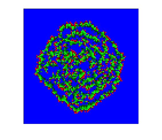
Imagine that the Wellesley College community has been quarantined due to a sudden outbreak of an annoying stomach virus. How quickly can this virus spread through the population, and will it eventually die out? This depends on factors such as the ease with which the virus is passed from one individual to another, the time it takes to recover from the virus, and the time during which an individual remains immune to the virus after recovering. One of the simplest models of the spread of disease was developed by W. O. Kermack and A. G. McKendrick in 1927 and is known as the SIR model. Its name is derived from the three populations it considers: Susceptibles (S) have no immunity from the disease, Infecteds (I) have the disease and can spread it to others, and Recovereds (R) have recovered from the disease and are immune to it.
In this problem, you will model the spread of a virus over time, through a population that is represented on a two-dimensional grid. Suppose that each cell on a 100x100 grid is an individual in a group of 10,000 people. Each individual can be susceptible, infectious or immune. Assume that the infection lasts two days and immunity lasts 5 days before the individual becomes susceptible again. The state of this virus in the population can be stored in a 100x100 matrix that contains values from 0 to 7 representing the following conditions:
The virus.m code file in the assign4_programs folder contains
partial code for a function named virus that simulates the spread of
the virus through the population, over a period of days.
The virus function has two inputs: the number of days to run the simulation,
and the probability that a susceptible individual will become infected if one of their
neighbors is infected. The function also has one output: a movie of the spread of the
virus from day to day. The 100x100 matrix grid1 is filled with the initial
state of the simulation on day 1, in which all of the individuals are susceptible, except
for a single infected individual in the center of the grid. The function
displayGrid, also provided in the assign4_programs folder,
displays the current grid as a color image. Susceptible individuals are shown in blue,
infected individuals are bright red on the first day and dark red on the second, and
recovered individuals are shown in shades of green from bright (value 3, first day of
recovery) to dark (value 7, fifth day after recovery). The code in the
virus function displays the initial grid on
day 1 and creates a snapshot of the grid display that is stored in the first frame
of the movie.
Your task is to complete the virus function to simulate the spread of the
virus, starting with day 2 and continuing over the input number of days. The function
should add a frame to the movie for each day of the simulation. A second 100x100 matrix
named grid2 is created in the initial code, to assist with the simulation. For
each new day, assume that the current state of the virus is stored in grid1.
Loop through all of the locations of grid1 (individuals in the population),
compute the new value for each individual and store it in the same location of grid2.
For example, if the value in grid1 at a particular location is 0 (susceptible
individual) and one of the neighbors (above, below, left or right) is infected (i.e. has the
value 1 or 2), then the input probability probInfect should be used to
determine whether the value stored at this location in grid2 should be a 0
(individual remains susceptible) or 1 (individual becomes infected). For each of the other
values stored in grid1, from 1 to 7, think about what value should be stored in
grid2 reflecting the state of the individual on the next day. (Remember that
immunity from the virus lasts for only 5 days after recovery, before the individual
becomes susceptible again.) Display the new grid with the displayGrid function
and use getframe to create a new
frame to add to the movie. After each day of the simulation is complete, copy the contents of
grid2 into grid1 in preparation for the next day of the simulation.
To simplify the task of checking whether a neighbor is infected, assume that there is a border
of individuals around the grid (rows 1 and 100, and columns 1 and 100) that remain susceptible
(value 0) throughout the simulation. When looping through grid1, you only need
to consider individuals in the rows and columns 2 through 99. Finally, the rand
function can be used to determine whether a susceptible individual with an infected
neighbor, becomes infected themselves. The function call rand(1) returns a
single random number between 0.0 and 1.0. Suppose we want to simulate the flipping
of a coin that is biased towards heads so that on average, 60% of the flips come up heads.
The following loop simulates 100 flips of this coin using a probability of 0.6:
for flips = 1:100
   if (rand(1) <= 0.6)
       disp('heads');
   else
       disp('tails');
   end
end
An analogous strategy can be used to determine whether a susceptible individual becomes
infected. When your virus function is complete, you can create and display a movie
of the spread of the virus. In the following example, the simulation is run for 60 days,
with a probability of infection of 0.5, and the movie is then viewed three times, with frames
presented at a rate of two frames per second:
>> myVirusMovie = virus(60,0.5);

>> movie(myVirusMovie, 3, 2);
The final frame of this movie might look something like this:
Run simulations for a few different values of the probablity (for example, 0.25, 0.5,
0.75, 1.0) and add some brief comments to the virus.m code file about
what you observe.