
bwlabel() bwlabel identifies parts of a binary matrix that are connected.
There is an optional second argument to bwlabel that is either 4 or 8.
With a second argument of 4, bwlabel looks for objects connected along
the four directions shown (up,down,left,right). With a second argument of 8,
bwlabel looks for objects connected along the diagonal as well as
those along the standard up, down, left and right directions.
 |
 |
bwlabel(BW,4) finds connections in these 4 directions |
bwlabel(BW,8) finds connections in these 8 directions |
Note: colors are used in the example above to illustrate how
BW = [ 1  1  1  0  0  0  0  0  0
       1  1  1  0  0  1  1  0  0
       1  1  1  0  0  1  1  0  0
       1  1  1  0  1  1  1  0  0
       1  1  1  0  0  0  0  1  1
       0  0  0  0  0  0  0  1  1
       0  0  0  0  0  0  1  1  1
       0  0  0  0  0  0  0  1  1  ];

L = bwlabel(BW,4)

L =  [ 1  1  1  0  0  0  0  0  0
       1  1  1  0  0  2  2  0  0
       1  1  1  0  0  2  2  0  0
       1  1  1  0  2  2  2  0  0
       1  1  1  0  0  0  0  3  3
       0  0  0  0  0  0  0  3  3
       0  0  0  0  0  0  3  3  3
       0  0  0  0  0  0  0  3  3  ];


Ls = bwlabel(BW,8)

Ls = [ 1  1  1  0  0  0  0  0  0
       1  1  1  0  0  2  2  0  0
       1  1  1  0  0  2  2  0  0
       1  1  1  0  2  2  2  0  0
       1  1  1  0  0  0  0  2  2
       0  0  0  0  0  0  0  2  2
       0  0  0  0  0  0  2  2  2
       0  0  0  0  0  0  0  2  2  ];
bwlabel works.
bwlabel identifies objects only by number; not color.
imshow(image,[min
max])
>> block(20:40,20:40) = 1; % intending to set a subsection to white
>> imshow(block); % hmmm, where is the white part??
>> block = uint8(zeros(50,50));
>> imshow(block);

>> imshow(block,[0,1]); % ahhh! There it is! 
imshow(X,map)
Colormaps and bwlabel mesh particularly well together. The labels that
bwlabel returns serve as indices into the colormap, creating what is called an
indexed image. Here is an
example:
X = [1  1  0  0  0  0  0  0  0  0
     1  1  0  0  0  0  0  0  0  0
     0  0  2  2  0  0  0  0  0  0
     0  0  2  2  0  0  0  0  0  0
     0  0  0  0  3  3  0  0  0  0
     0  0  0  0  3  3  0  0  0  0
     0  0  0  0  0  0  4  4  0  0
     0  0  0  0  0  0  4  4  0  0
     0  0  0  0  0  0  0  0  5  5
     0  0  0  0  0  0  0  0  5  5];

 redmap = zeros(5,3);
 redmap(1,1)= 0.20;
 redmap(2,1)= 0.40;
 redmap(3,1)= 0.60;
 redmap(4,1)= 0.80;
 redmap(5,1)= 1.0;

>> redmap
redmap =
    0.2000         0         0
    0.4000         0         0
    0.6000         0         0
    0.8000         0         0
    1.0000         0         0

% making a greenish bluish map
 aquamap = zeros(5,3);
 aquamap(1,2) = 0.20;
 aquamap(1,3) = 0.20;
 aquamap(2,2) = 0.40;
 aquamap(2,3) = 0.40;
 aquamap(3,2) = 0.60;
 aquamap(3,3) = 0.60;
 aquamap(4,2) = 0.80;
 aquamap(4,3) = 0.80;
 aquamap(5,2) = 1.0;
 aquamap(5,3) = 1.0;

>> aquamap
 aquamap =
         0    0.2000    0.2000
         0    0.4000    0.4000
         0    0.6000    0.6000
         0    0.8000    0.8000
         0    1.0000    1.0000
>>
We can display the image X above by specifying a display range as the second input: imshow(X) to produce?
>> imshow(X, [0 5]);

Or, we could display it with the colormap redmap:
>> imshow(X,redmap);

With the redmap colormap, the labels in the image X correspond to rows in
the colormap from top to bottom. So the first label 1 (in the upper left corner)
takes the color from the first row of redmap which is [0.20 0 0] which is a
pale red. This pattern continues, with the last label 5 (in the lower right corner)
taking the color from the fifth row of redmap which is [1.0 0 0] or pure red.
Or, we could display it with the colormap aquamap:
>> imshow(X,aquamap);

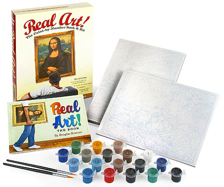
An analogy that is often used for indexed images is that of paint-by-numbers. The image has areas with color indicated by different numbers. Each paint tub has a number on it, linking the colors and the numbers in the image. The same thing is happening here with the labeled image and the colormap, although the indexing is implicit (row i of the colormap corresponds to the ith label in the image).
Notes:
redmap colormap above set values for only the first column because
variations of red were desired. For other colors, any combination of the red/green/blue
(first/second/third columns) can be manipulated.