CS112: More on 2-D Visualization

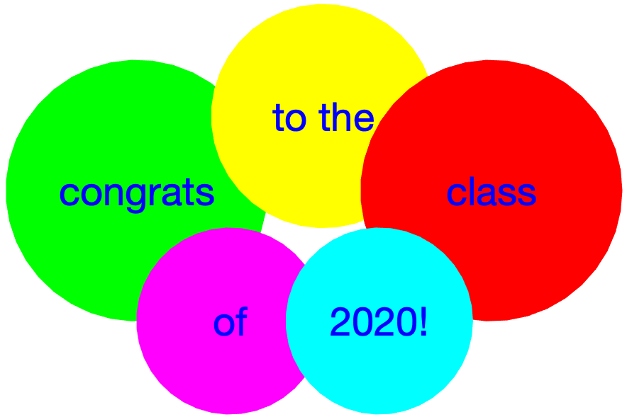
% CLASS OF 2020 BALLOONS
hold on
colors = 'gyrmc';
strings = {'congrats' 'to the' 'class' 'of' '2020!'};
xpos = [0 50 95 25 65];
ypos = [60 80 60 25 25];
rads = [35 30 35 25 25];
for i = 1:5
    drawBubble(xpos(i), ypos(i), rads(i), colors(i), strings{i});
end
axis equal off

function drawBubble (xcenter, ycenter, radius, color, string)
% draw circle with input xcenter, ycenter, radius, color and text
angles = linspace(0, 2*pi, 40);
bubx = xcenter + (radius * cos(angles));
buby = ycenter + (radius * sin(angles));
fill(bubx, buby, color, 'EdgeColor', color)
text(xcenter, ycenter, string, 'Color', [0 0 1], 'FontSize', 28, ...
       'FontWeight', 'normal', 'HorizontalAlignment', 'center')

Pie chart

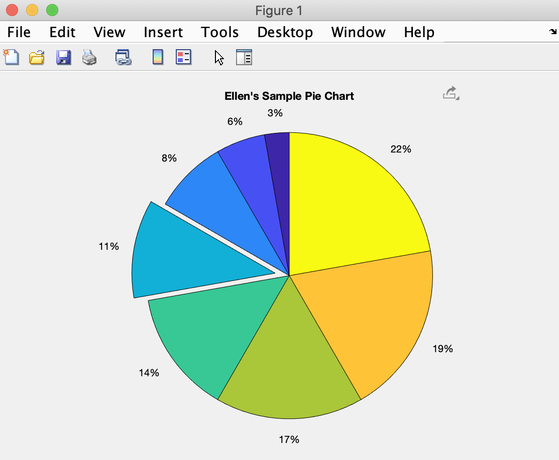
% PIE CHART
slices = [5 10 15 20 25 30 35 40];
pullout = [0 0 0 1 0 0 0 0];
pie(slices, pullout);     % pull out one of the slices
title('Ellen''s Sample Pie Chart');

Bar graph

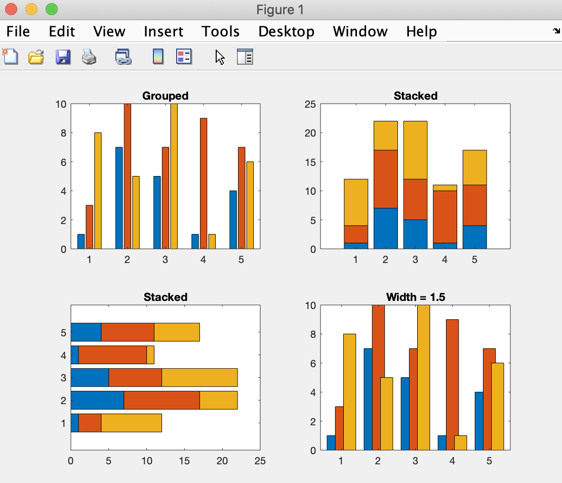
% BAR GRAPHS
% data is a 5x3 matrix, to create 5 groups of 3 bars
data = [1 3 8; 7 10 5; 5 7 10; 1 9 1; 4 7 6];
subplot(2,2,1)
bar(data,'grouped')     % groups of vertical bars
title('Grouped')
subplot(2,2,2) 
bar(data,'stacked')     % stacked areas
title('Stacked')
subplot(2,2,3)
barh(data,'stacked')    % horizontal bars
title('Stacked')
subplot(2,2,4)
bar(data, 1.5)          % wider bars
title('Width = 1.5')

Error bars

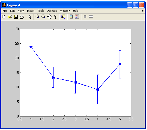
% ERROR BARS
load hogg
% hogg =
%     24    14    11     7    19
%     15     7     9     7    24
%     21    12     7     4    19
%     27    17    13     7    15
%     33    14    12    12    10
%     23    16    18    18    20
means = mean(hogg);     % mean values for columns
stds = std(hogg);       % standard deviations for columns
errorbar(means, stds, 'b*-', 'MarkerSize', 10, 'LineWidth', 2);

Box plot

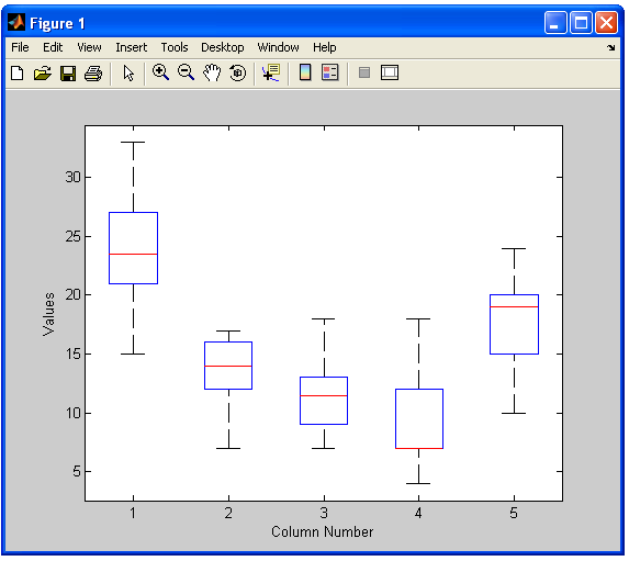
% BOX PLOT
boxplot(hogg)

Histograms

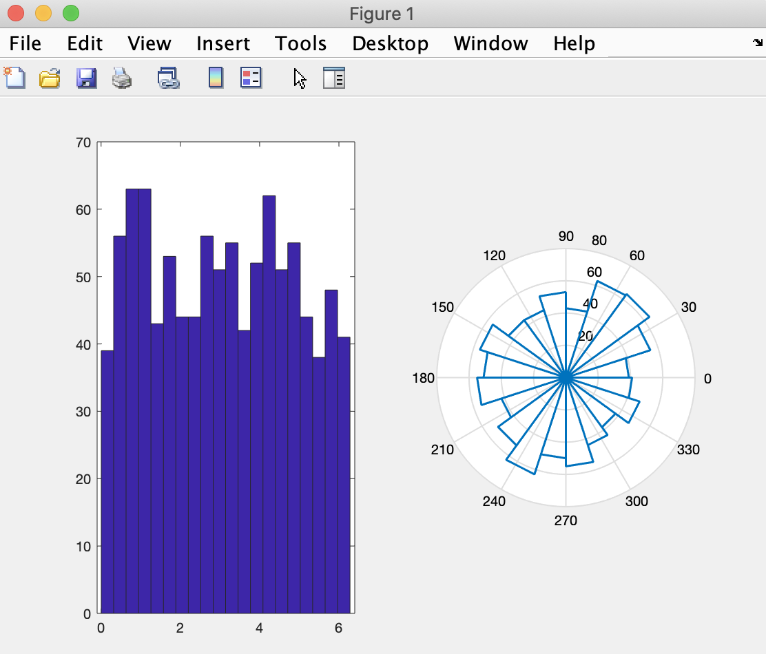
% HISTOGRAMS
% 1000 random angles from 0 to 2pi
angles = 2*pi*rand(1,1000);
subplot(1,2,1)
hist(angles, 20)        % linear histogram
axis([-0.1 6.4 0 70])
subplot(1,2,2)
rose(angles, 20)        % angular histogram
hline = findobj(gca, 'Type', 'line');
set(hline, 'LineWidth', 1.5)

Stem plot

% STEM PLOT
x = 0:0.1:4;
y = sin(x.^2) .* exp(-x);
stem(x, y, 'fill')

Staircase plot

% STAIRCASE PLOT
stairs(x, y, 'LineWidth', 2)

Polar plot

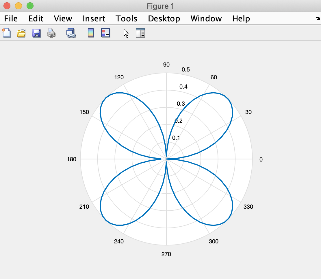
% POLAR PLOT
angles = linspace(0, 2*pi, 100);
polar(angles, abs(sin(angles).*cos(angles)))
hline = findobj(gca, 'Type', 'line');
set(hline, 'LineWidth', 2)

Compass plot

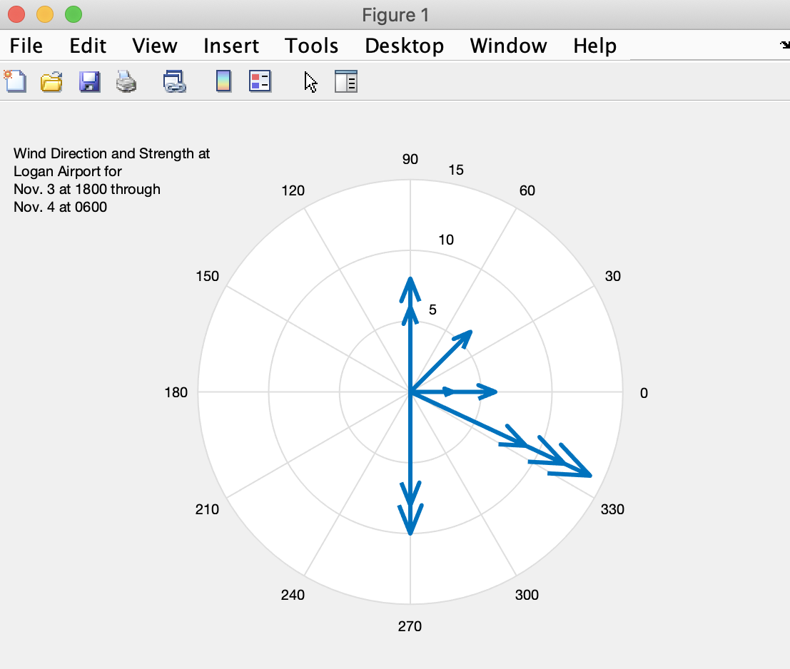
% COMPASS PLOT
% wind directions in degrees for a 12-hour period
wdir = [45 90 90 45 360 335 360 270 335 270 335 335];
knots = [6 6 8 6 3 9 6 8 9 10 14 12];   % wind speeds
rdir = wdir * pi/180;                   % convert to radians
[x,y] = pol2cart(rdir,knots);
compass(x,y)
hline = findobj(gca, 'Type', 'line');
set(hline, 'LineWidth', 3)
desc = {'Wind Direction and Strength at',
        'Logan Airport for ',
        'Nov. 3 at 1800 through',
        'Nov. 4 at 0600'};
text(-28,15,desc)

Vector plot

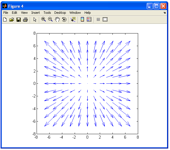
% VECTOR PLOT
[X Y] = meshgrid(-5:5);   % coordinates for vector positions
VX = X/5;                 % X,Y components of vector
VY = Y/5;                 
quiver(X, Y, VX, VY, 2)
axis square

Fancy text

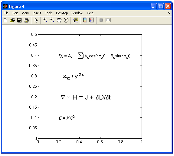
% FORMATTED TEXT
% example from Hanselman & Littlefield, MASTERING MATLAB 7
axis([0 1 0 0.5])
text(0.2, 0.1, '\itE = M\cdotC^{\rm2}')
text(0.2, 0.2, '\fontsize{16} \nabla \times H = J + \partialD/\partialt')
text(0.2, 0.3, '\fontname{courier}\fontsize{16}\bf x_{\alpha}+y^{2\pi}')
str1 = 'f(t) = A_o + \fontsize{30}_\Sigma\fontsize{10}';
text(0.2, 0.4, [str1 '[A_ncos(n\omega_ot) + B_nsin(n\omega_ot)]'])

For more information about adding text, search for Text Properties in the MATLAB Help pages.

Log axes

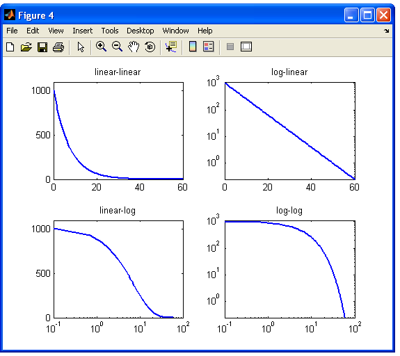
% LOG AXES
x = linspace(0.1,60,100);
y = 2.^(-0.2*x+10);
subplot(2,2,1)
plot(x, y, 'LineWidth', 2)
title('linear-linear')
axis([0 60 0 1100])
subplot(2,2,2)
semilogy(x, y, 'LineWidth', 2)
title('log-linear')
axis([0 60 0 1100])
set(gca, 'YTick', [0.1 1 10 100 1000])
subplot(2,2,3)
semilogx(x, y, 'LineWidth', 2)
title('linear-log')
axis([0 100 0 1100])
set(gca, 'XTick', [0.1 1 10 100]);
subplot(2,2,4)
loglog(x, y, 'LineWidth', 2)
title('log-log')
set(gca, 'XTick', [0.1 1 10 100]);
set(gca, 'YTick', [0.1 1 10 100 1000])
axis([0 100 0 1100])