Reading: Bézier Curves¶

This reading is organized as follows. First, we look at why we try to represent curves and surfaces in graphics models, but I think most of us are already pretty motivated by that. Then, we look at major classes of mathematical functions, discussing the pros and cons, and finally choosing cubic parametric equations. Next, we describe different ways to specify a cubic equation, and we ultimately settle on Bézier curves. Finally, we look at how the mathematical tools that we've discussed are reflected in WebGL/Three.js code.

The preceding develops curves (that is, 1D objects — wiggly lines). In graphics, we're mostly interested in surfaces (that is, 2D objects — wiggly planes). Next time, we'll look at how to define surfaces as a generalization of what we've already done with curves.

Introduction¶

Bézier curves were invented by a mathematician working at Renault, the French car company. He wanted a way to make formal and explicit the kinds of curves that had previously been designed by taking flexible strips of wood (called splines , which is why these mathematical curves are often called splines) and bending them around pegs in a pegboard. To give credit where it's due, another mathematician named de Castelau independently invented the same family of curves, although the mathematical formalization is a little different.

Representing Curves¶

We all know about different kinds of curves, such as parabolas, circles, the square root function, cosines and so forth. Most of those curves can be represented mathematically in several ways:

• explicit equations
• implicit equations
• parametric equations

Explicit Equations¶

The explicit equations are the ones we're most familiar with. For example, consider the following functions:

$$ \begin{array}{rcl} y &=& mx+b\\ y &=& ax^2+bx+c\\ y &=& \sqrt{r^2-x^2}\\ \end{array} $$

An explicit equation has one variable that is dependent on the others; here it is always $y$ that is the dependent variable: the one that is calculated as a function of the others.

An advantage of the explicit form is that it's pretty easy to compute many values on the curve: just iterate $x$ from some minimum to some maximum value.

One trouble with the explicit form is that there are often special cases (for example, vertical lines). Another is that the limits on $x$ will change from function to function (the domain is infinite for the first two examples, but limited to $\pm r$ for the third). The deadly blow is that it's hard to handle non-functions, such as a complete circle, or a parabola of the form $x=ay^2+by+c$. You could certainly get a computer program to handle this form, but you'd need to encode lots of extra stuff, like which variable is the dependent one and so forth. Bézier curves can be completely specified by just an array of coefficients.

Implicit Equations¶

Another class of representations are implicit equations. These equations always put everything on one side of the equation, so no variable is distinguished as the dependent one. For example:

$$ \begin{array}{rcl} ax+by+cz-d=0 & & \textrm{plane} \\ ax^2+by^2+cz^2-d^2=0 & & \textrm{egg} \\ \end{array} $$

These equations have a nice advantage that, given a point, it's easy to tell whether it's on the curve or not: just evaluate the function and see if the function is zero. Moreover, each of these functions divides space in two: the points where the function is negative and the points where it's positive. Interestingly, the surfaces do as well, so the sign of the function value tells you which side of the surface you're on. (It can even tell you how close you are.)

The fact that no variable is distinguished helps to handle special cases. In fact, it would be pretty easy to define a large general polynomial in $x$, $y$ and $z$ as our representation.

The deadly blow for this representation, though, is that it's hard to generate points on the surface. Imagine that I give you a value for $a$, $b$, $c$ and $d$ and you have to find a value for $x$, $y$, and $z$ that work for the two examples above. Not easy in general. Also, it's hard to do curves (wiggly lines). In general, curves are the intersection of two surfaces, like conic sections (parabola, ellipse, etc.) being the intersection of a cone and a plane.

Parametric Equations¶

Finally, we turn to the parametric equations. We've seen these before, of course, in defining lines, which are just straight curves.

With parametric equations, we invent some new variables, parameters , typically $s$ and $t$. These variables are then used to define a function for each coordinate:

\[ \vecIII{x(s,t)}{y(s,t)}{z(s,t)} \]

Parametric functions have the advantage that they're easy to generalize to 3D, as we already saw with lines.

The parameters tell us where we are on the surface (or curve) rather than where we are in space. Therefore, we have a conventional domain, namely the unit interval. This means that, like our line segments, our curves will all go from $t=0$ to $t=1$. (They don't have to, but they almost always do.) Similarly, surfaces are all points where $0\leq s,t \leq 1$. Thus, another advantage of parametric equations is that it's easy to define finite segments and sheets, by limiting the domains of the parameters.

The problem that remains is what family of functions we will use for the parametric functions. One standard approach is to use polynomials, thereby avoiding trigonometric and exponential functions, which are expensive to compute. In fact, we usually choose a cubic:

$$ \begin{array}{rcl} x(t) &=& C_0+C_1 t + C_2 t^2 + C_3 t^3 \\ &=& \sum_{i=0}^{3} C_i t^i \end{array} $$

Another problem comes with finding these coefficients. We'll develop this in later sections, but the solution is essentially to appeal to some nice techniques from linear algebra that let us solve for the desired coefficients given some desired constraints on the curve, such as where it starts and where it stops.

Why We Want Low Degree¶

Why do we typically use a cubic? Why not something of higher degree, which would let us have more wiggles in our curves and surfaces? This is a reasonable question.

In general, we want a low degree: quadratic, cubic or something in that neighborhood. There are several reasons:

1. The resulting curve is smooth and predictable over long spans. In other words, because it wiggles less, we can control it more easily. Consider trying to make a nice smooth curve with a piece of cardboard or thin wood (a literal spline) versus with a piece of string.
2. It takes less information to specify the curve. Since there are four unknown coefficients, we need four points (or similar constraints) to solve for the coefficients. If we were using a quartic, we'd need 5 points, and so forth.
3. If we want more wiggles, we can join up several splines. Because of the low degree, we have good control of the derivative at the end points, so we can make sure that the curve is smooth through the joint.
4. Finally, it's just less computation and therefore easier for the program to render.

OpenGL/WebGL will permit you to use higher (and lower) degree functions, but for this presentation we'll stick to cubics.

Ways of Specifying a Curve¶

Once we've settled on a family of functions, such as cubics, what remains is determining the values of the coefficients that give us a particular curve. To define a cubic, we need four pieces of information, though there are different choices about what four pieces of information. If we want, for example, a curve that looks like the letter "J," what four pieces of information do we need to specify? It turns out that there are three major ways of doing this. (It's strange how everything seems to break down into threes in this subject.)

• Interpolation: That is, you specify four points on the curve and the curve goes through (interpolates) the points. This is pretty intuitive, and a lot of drawing programs allow you to do this, but it's not often used in CG. This is primarily because such curves have an annoying way of suddenly lurching as they struggle to get through the next specified point.¹
• Hermite: In the Hermite case, the four pieces of information you specify are 2 points and 2 vectors: the points are where the curve starts and ends, and the vectors indicate the direction of the curve at that point. They are, in fact, derivatives. (If you've done single-dimensional calculus, you know that the derivative gives the slope at any point and the slope is just the direction of the line; the same idea holds in more dimensions.) This is a very important technique, because we often have this information. For example, if I want a nice rounded corner on a square box, I know the slope at the beginning (vertical, say) and at the end (horizontal).
• Bézier: With a Bézier curve, we specify 4 points, as follows: the curve starts at the first point, heading for the second, ends at the fourth, coming from the third (see the picture below). This is a very important technique, because you can easily specify a point using a GUI, while a vector is a little harder. It turns out there are other reasons that Bézier is preferred, and in practice the first two techniques are implemented by finding the Bézier points that draw the desired curve.

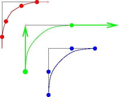
The figure above compares these three approaches.

OpenGL/WebGL curves are drawn by calculating points on the line and drawing straight line segments between those points. The more segments, the smoother the resulting curve looks. In some implementations, the calculations can be done by the graphics card. In Three.js, they compute the vertices in the main processor, rather than having the graphics card do this. It may be because they want to simplify the shader program, but that's a guess.

Defining a Bezier Curve¶

The following figure shows four points defining a Bezier curve.

Fun fact: the curve above is not an image. It is a Bezier curve drawn using the 2D WebGL API.

Joining Curves¶

To make longer curves with more wiggles, we can join up several Bézier curves. The following figure shows two examples. In each subfigure, the first curve (in green) is defined by 4 points: P0, P1, P2, P3; the second curve (in red) is defined by 4 points: Q0, Q1, Q2, Q3.

In the first subfigure, the curves are connected (the last control point of the first curve is the same as the first point of the second), but not smooth through the joint. The second subfigure manages to make the joint smooth, by making sure the tangents line up.

How do we make the tangents line up, creating a smooth joint? The tangents are defined by the line segments from P2 to P3 and from Q0 to Q1. So, the joint will be smooth if these three points are co-linear (form a line):

P2, P3==Q0, Q1

You'll notice in the second subfigure above, P3 is the same as Q0, and P2, P3=Q0 and Q2 form a straight line. In fact, the distance from P2 to P3 is the same as the distance from Q0 to Q1.

Solving for the Coefficients¶

We'll now discuss how we can solve for the coefficients given the control information (the four points or the two points and two vectors). Essentially, we're solving four simultaneous equations. We won't do all the gory details, but we'll appeal to some results from linear algebra.

Let's look at how we solve for the coefficients in the case of the interpolation curves; the others work similarly.

Note that in every case, the parameter is $t$ and it goes from $0$ to $1$. For the interpolation curve, the interior points are at $t=1/3$ and $t=2/3$. Let's focus just on the function for $x(t)$. The other dimensions work the same way. If we substitute $t=\{0, \frac13, \frac23, 1 \}$ into the cubic equations we saw earlier, we get the following:

$$ \begin{array}{lclcl} P_0 &=& x(0) &=& C_0 +C1\cdot0 + C2\cdot0+C3\cdot0\\ P_1 &=& x(1/3) &=& C_0+\frac13C_1 + \left(\frac13\right)^2C_2 + \left(\frac13\right)^3C_3\\ P_2 &=& x(2/3) &=& C_0+\frac23C_1 + \left(\frac23\right)^2C_2 + \left(\frac23\right)^3C_3\\ P_3 &=& x(1) &=& C_0+C_1\cdot1 + C_2\cdot1 + C_3\cdot1\\ \end{array} $$

What does this mean? It means that the $x$ coordinate of the first point, $P_0$, is $x(0)$. This makes sense: since the function $x$ starts at $P_0$, it should evaluate to $P_0$ at $t=0$. (This is also exactly what happens with a parametric equation for a straight line: at $t=0$, the function evaluates to the first point.) Similarly, the $x$ coordinate of the second point, $P_1$ is $x(1/3)$ and that evaluates to the expression that you see there. Most of those coefficients are still unknown, but we'll get to how to find them soon enough.

Putting these four equations into a matrix notation, we get the following:

\[ \mathbf{P} = \left[ \begin{array}{cccc} 1 & 0 & 0 & 0 \\ 1 & \frac13 & (\frac13)^2 & (\frac13)^3 \\ 1 & \frac23 & (\frac23)^2 & (\frac23)^3 \\ 1 & 1 & 1 & 1 \\ \end{array}\right] \mathbf{C} \]

The $\mathbf{P}$ matrix is a matrix of points. It could just be the $x$ coordinates of our points $P$, or more generally it could be a matrix each of whose four entries is an $(x,y,z)$ point. We'll view it as a matrix of points. The matrix $\mathbf{C}$ is a matrix of coefficients , where each element — each coefficient — is a triple $(C_x,C_y,C_z)$, meaning the coefficients of the $x(t)$ function, the $y(t)$ function, and the $z(t)$ function.

If we let $\mathbf{A}$ stand for the array of numbers, we get the following deceptively simple equation:

\[ \mathbf{P} = \mathbf{A} \mathbf{C} \]

By inverting the matrix $\mathbf{A}$, we can solve for the coefficients! (The inverse of a matrix is the analog to a reciprocal in scalar mathematics. It's also equivalent to solving the simultaneous equations in a very general way.) The inverse of $\mathbf{A}$ is called the interpolating geometry matrix and is denoted $\mathbf{M}_I$:

\[ \mathbf{M}_I = \mathbf{A}^{-1} \]

Notice that the matrix $\mathbf{M}_I$ does not depend on the particular points we choose, so that matrix can simply be stored in our program somewhere. When we need to calculate points on the curve, we compute the necessary coefficients:

\[ \mathbf{C} = \mathbf{M}_I \mathbf{P} \]

The same approach works with Hermite and Bézier curves, yielding the Hermite geometry matrix and the Bézier geometry matrix. In the Hermite case, we take the derivative of the cubic and evaluate it at the endpoints and set it equal to our desired vector (instead of points $P_1$ and $P_2$). In the Bézier case, we use a point to define the vector and reduce it to the previously solved Hermite case.

Blending Functions¶

Sometimes, looking at the function in a different way can give us additional insight. Instead of looking at the functions in terms of control points and geometry matrices, let's look at them in terms of how the control points influence the curve points.

Looking just at the functions of $t$ that are combined with the control points, we can get a sense of the influence each control point has over each curve point. The influences of the control points are blended to yield the final curve point, and these functions are called blending functions. (Blending functions are also important for understanding NURBS, a generalization of Bézier curves.) Equivalently, the curve points are a weighted average of the control points, where the blending functions give the weight. That is, if you evaluate the four blending functions at a particular parameter value, $t$, you get four numbers, and those numbers are weights in a weighted sum of the four control points.

The following function gives the curve, $P(t)$, as a weighted sum of the four control points, where the four blending functions evaluate to the appropriate weight as a function of $t$.

$$ P(t) = B_0(t)\cdot P_0 + B_1(t)\cdot P_1 + B_2(t)\cdot P_2 + B_3(t)\cdot P_3 $$

The following are the blending functions for interpolating curves.

\begin{array}{rcl} B_0(t) &=& \frac{-9}2(t-\frac13)(t-\frac23)(t-1) \\ B_1(t) &=& \frac{27}2t(t-\frac23)(t-1) \\ B_2(t) &=& \frac{-27}2t(t-\frac13)(t-1) \\ B_3(t) &=& \frac{-9}2t(t-\frac13)(t-\frac23) \\ \end{array}

These functions are plotted in the following figure:

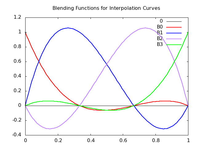
Alternatively, you can go over to Wolfram Alpha and see the live plotting (and adjust to your taste) by clicking on these links

plot (-9/2)(t-(1/3))(t-(2/3))(t-1) from t=0 to 1

plot (-9/2)(t-(1/3))(t-(2/3))(t-1), (27/2)t(t-(2/3))(t-1), (-27/2)t(t-(1/3))(t-1) from t=0 to 1

plot (-9/2)(t-(1/3))(t-(2/3))(t-1), (27/2)t(t-(2/3))(t-1), (-27/2)t(t-(1/3))(t-1), (-9/2)t(t-(1/3))(t-(2/3)) from t=0 to 1

plot (-9/2)(t-(1/3))(t-(2/3))(t-1), (27/2)t(t-(2/3))(t-1), (-27/2)t(t-(1/3))(t-1), (-9/2)t(t-(1/3))(t-(2/3)) from t=0 to 1

First, notice that the curves always sum to 1. (It may not be entirely obvious, but it's true.) When a curve is near zero, the control point has little influence. When a curve is high, the weight is high and the associated control point has a lot of influence: a lot of "pull." In fact, when a control point has a lot of pull, the curve passes near it. When a weight is 1, the curve goes through the control point.

Notice that the blending functions are negative sometimes (they all start and end at zero), which means that this isn't a normal weighted average. (A normal weighted average has all non-negative weights.) What would a negative weight mean? If a positive weight means that a control point has a certain "pull," a negative value gives it "push" — the curve is repelled from that control point. This repulsion effect is part of the reason that interpolation curves are hard to control.

Hermite Representation¶

The coefficients for the Hermite curves and therefore the blending functions can be computed from the control points in a similar way (we have to deal with derivatives, but that's not the point right now).

Note that the derivative (tangent) of a curve in 3D is a 3D vector , indicating the direction of the curve at this moment. (This follows directly from the fact that if you subtract two points, you get the vector between them. The derivative of a curve is simply the limit as the points you're subtracting become infinitely close to each other.)

The Hermite blending functions are the following.

\[ \mathbf{b}(t) = \vecIV{2t^3-3t^2+1} {-2t^3+3t^2} {t^3-2t^2+t} {t^3-t^2} \]

The Hermite blending functions are plotted in the following figure:

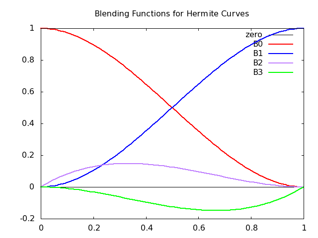
The Hermite curves have several advantages:

• Smoothness:
  • It's easier to join up at endpoints. Because we control the derivative (direction) of the curve at the endpoints, we can ensure that when we join up two Hermite curves that the curve is smooth through the joint: just ensure that the second curve starts with the same derivative that the first one ends with.
  • The blending functions don't have zeros in the interval: so the influence of a control point never switches from positive to negative. For example, the influence of the first control point peaks at the beginning and steadily, monotonically, drops to zero over the interval.
• Control:
  • The Hermite can be easier to control. As we mentioned earlier, there's no need to know interior points, and we often only know how we want a curve to start and end.

Bézier Curves¶

The Bézier curve is based on the Hermite, but instead of using vectors, we use two control points. Those control points are not interpolated though: they exist only in order to define the vectors for the Hermite, as follows:

\begin{array}{rcl} p'(0) &=& \frac{p_1-p_0}{1/3} = 3(p_1-p_0)\\ p'(1) &=& \frac{p_3-p_2}{1/3} = 3(p_3-p_2) \end{array}

That is, the derivative vector at the beginning is just three times the vector from the first control point to the second, and similarly for the other vector. The figure below shows the derivative vectors and the Bézier control points. Notice (as we can see from the equations above), that the vectors are three times longer than the distance of the inner control points from the end control points. However, that's not important. The factor is chosen so that the resulting equations are simplified.

Like the Hermite, Bézier curves are easily joined up. We can easily get continuity through a joint by making sure that the last two control points of the first curve line up with the first two control points of the next. Even better, the interior control points should be equally distant from the joint. This ensures that the derivatives are equal and not just proportional. You can see this in the earlier figure where we smoothly joined two Bézier curves

Repeating that figure:

• The last control point of the green curve (P3) is the same as the first point of the red curve (Q0).
• The three points (P2, P3=Q0, Q1) form a straight line. (In this case it's a vertical line, but that was just for convenience.) This co-linearity means that the derivatives are in the same direction, so the joint is smooth.
• The distance from P2-P3 is the same as the distance from Q0-Q1, so that the derivatives are not just lined up but are actually equal. This gives extra smoothness.

The Bézier blending functions are especially nice, as seen in the following equation:

Here is a figure that plots the Bézier blending functions:

These blending functions are from a family of functions called the Bernstein polynomials:

\[ b_{kd}(t) = \Choose{d}{k} t^k(1-t)^{d-k} \]

These can be shown to:

• have all roots at 0 and 1
• be non-negative in the interval [0,1]
• be bounded by 1
• sum to 1

Perfect for mixing! Just like the points on a line segment can be viewed as a mixture (weighted sum) of the two endpoints, we can think of each point on a Bezier curve as a mixture of its four control points!

Convex Hull¶

Our Bézier curve is a weighted sum, so geometrically, all points must lie within the convex hull of the control points, as shown in the following figure. (The convex hull is like the bounding boxes we discussed: a set of points such that the curve is entirely inside the convex hull.)

Examples: S Curves¶

Now that we understand the theory and therefore the meaning of these four control points, let's see some examples in Threejs.

Here is a simple S-shaped curve, lying flat in the Z=0 plane:

curves/s-curve1

Let's look at the code piece by piece. First, the control points:

var controlPoints = [
    [0,0,0],   // start at origin
    [2,2,0],   // head northeast, towards this point
    [-2,1,0],  // finish from west southwest, as if from this point
    [0,3,0],   // finish here
];

It's always a little weird (at least for me) to read these in order, because the third control point is not a destination, but instead controls from what direction you arrive at the last control point, which is a destination. I usually like to think about where I'm going and then think about how I get there. But we can get used to this fairly quickly.

Now, let's see how to draw a line using those control points. First, we have to create the geometry. The approach here is to create an object that will be able to compute any point on the curve. That object is an instance of CubicBezierCurve3 which is a subclass of Curve which has methods like getPoint(t) where t is a parameter from 0 to 1. Hopefully, the preceding theory discussion makes that perfectly cromulent.².

We will actually use another method, .getPoints(divisions) which returns an array of as many points as we request. Then, we store those points in the geometry object and return it.

Here's the code from the CubicBezierCurve3 documentation page:

const curve = new THREE.CubicBezierCurve3(
    new THREE.Vector3( -10, 0, 0 ),
    new THREE.Vector3( -5, 15, 0 ),
    new THREE.Vector3( 20, 15, 0 ),
    new THREE.Vector3( 10, 0, 0 )
);

const points = curve.getPoints( 50 );
const geometry = new THREE.BufferGeometry().setFromPoints( points );

const material = new THREE.LineBasicMaterial( { color: 0xff0000 } );

// Create the final object to add to the scene
const curveObject = new THREE.Line( geometry, material );

Note that in the code above, instead of using THREE.Mesh() to combine a geometry and a material, they use THREE.Line(). This is an important change for today's material. In practice we will rarely draw lines, we will usually be creating meshes. But for today: THREE.Line

In the documentation example, the control points are THREE.Vector3(), but I find that cumbersome. I like using nice nested arrays, like we saw above. Because our control points are in theses nested arrays, we'll need to transform them a bit. So, we'll use the following function. You'll notice in this code several uses of the JS syntax ...array which "spreads" an array into different values. See JS spread syntax. Here, it allows us to pass that array of vectors into a function that wants separate arguments for each control point:

function createBezierCurve(controlPoints, numPoints) {
    // turn each JS array into a Vector
    const vecs = controlPoints.map( a => new THREE.Vector3(...a) );
    // create the curve object with four control points
    const curve = new THREE.CubicBezierCurve3(...vecs);
    // sample the curve 
    const points = curve.getPoints(numPoints);
    const geo = new THREE.BufferGeometry();
    geo.setFromPoints(points);
    return geo;
}

Given the foregoing code, here's how we can draw our line:

// Unfortunately the linewidth is ignored in WebGL
const curveMat = new THREE.LineBasicMaterial( { color: "blue",
                                                linewidth: 5 } );

const curveGeo = createBezierCurve(controlPoints, 20);
const curve = new THREE.Line( curveGeo, curveMat );
scene.add(curve);

Once again, notice that we use THREE.Line here, not THREE.Mesh. I'm emphasizing that because it's easy to overlook, and when I did, it took a long time to debug.

Finally, just for visual feedback, it's nice to draw a tiny sphere at each control point, so we can see them:

// This creates a tiny sphere at each control point
function showCP(cpList) {
    for( var i=0; i < cpList.length; i++ ) {
        scene.add(TW.createPoint(cpList[i]));
    }
};

showCP(controlPoints);          // optional, for debugging.

S-Curve with TW helper¶

That createBezierCurve helper function looks to be useful and generic, so I added it to TW. Here's a demo that uses that helper function:

curves/s-curve-tw

Box Curve¶

The S-curve above is flat: lies in the Z=0 plane. A slightly more interesting curve is this one:

curves/box-curve

Move the camera a little to see it "pop" into 3D. Alternatively, turning on the bounding box will give a clue as to how this curve is moving through space.

I made a few other small changes to that example, including clearing the background to black (which usually makes the lines show more clearly).

TW.clearColor = 0x000000;       // clear to black
TW.mainInit(renderer,scene);

Coke Bottle Silhouette¶

As an example of a joining some curves together, I once created the silhouette of a coke bottle:

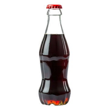
This silhouette requires three bends, and a single Bezier curve can really only have one bend in it, so I put three curves together to create the silhouette. The curves look like this:

// Upper curve, from diameter of 0.75in at height 5in to diameter of 1.5in
// at height 2.5in. 

const upperCP = [[0.5/2, 5.0, 0.0],
                 [0.5/2, 4.0, 0.0],
                 [1.5/2, 3.0, 0.0],
                 [1.5/2, 2.5, 0.0]];

// Middle curve, from upper bulge [see previous] to dent with diameter of
// 1.25in at height of 1.25in. */

const middleCP = [[1.5/2,  2.5,  0.0],
                  [1.5/2,  2.0,  0.0],
                  [1.25/2, 1.75, 0.0],
                  [1.25/2, 1.25, 0.0]];

// Lower curve, from dent to base, with a radius the same as the bulge. 

const lowerCP = [[1.25/2, 1.25, 0.0],
                 [1.25/2, 0.75, 0.0],
                 [1.5/2,  0.50, 0.0],
                 [1.5/2,  0.00, 0.0]];

I created this silhouette by measuring an actual coke bottle (though I think it might have been plastic and not glass). The distances are widths of the bottle, so to make it symmetrical around zero, I divided each x-coordinate in half. The y coordinates are distance in inches from the bottom of the bottle. Here's the demo:

curves/coke

When playing with it, be sure to try the options in the GUI:

• clicking allRed shows the middle curve in white, so you can easily see the three pieces
• clicking showControlPoints shows all 12 control points as yellow spheres

Summary¶

• We want to represent curves using mathematical functions, where we can easily calculate any point on the curve.
• Using polynomials of low degree is useful because:
  • we don't need a lot of control points to specify them
  • they aren't too "wiggly"; easy to control
  • they are relatively less expensive to compute
• We'll focus on cubics which require
  • the beginning and end points
  • the beginning and end vectors (directions)
• If we want more wiggles, we can join up several beziers
• Demos:
  • curves/s-curve1
  • curves/s-curve-tw
  • curves/box-curve
  • curves/coke