|
CS 332
Assignment 4 Due: Thursday, October 25 |
|
This assignment has one problem that builds on the algorithm proposed by Longuet-Higgins and
Prazdny to compute an observer's heading from the image velocity field generated from their
movement relative to the environment. To begin, download the /home/cs332/download/Assign4
folder and set the Current Folder in MATLAB to this folder. (Note that the folder contains updated
versions of some of the functions used in the Observer Motion Lab
that you started in a previous class — keep the two folders separate when working on this
assignment.) You are welcome to work with a partner on this problem.
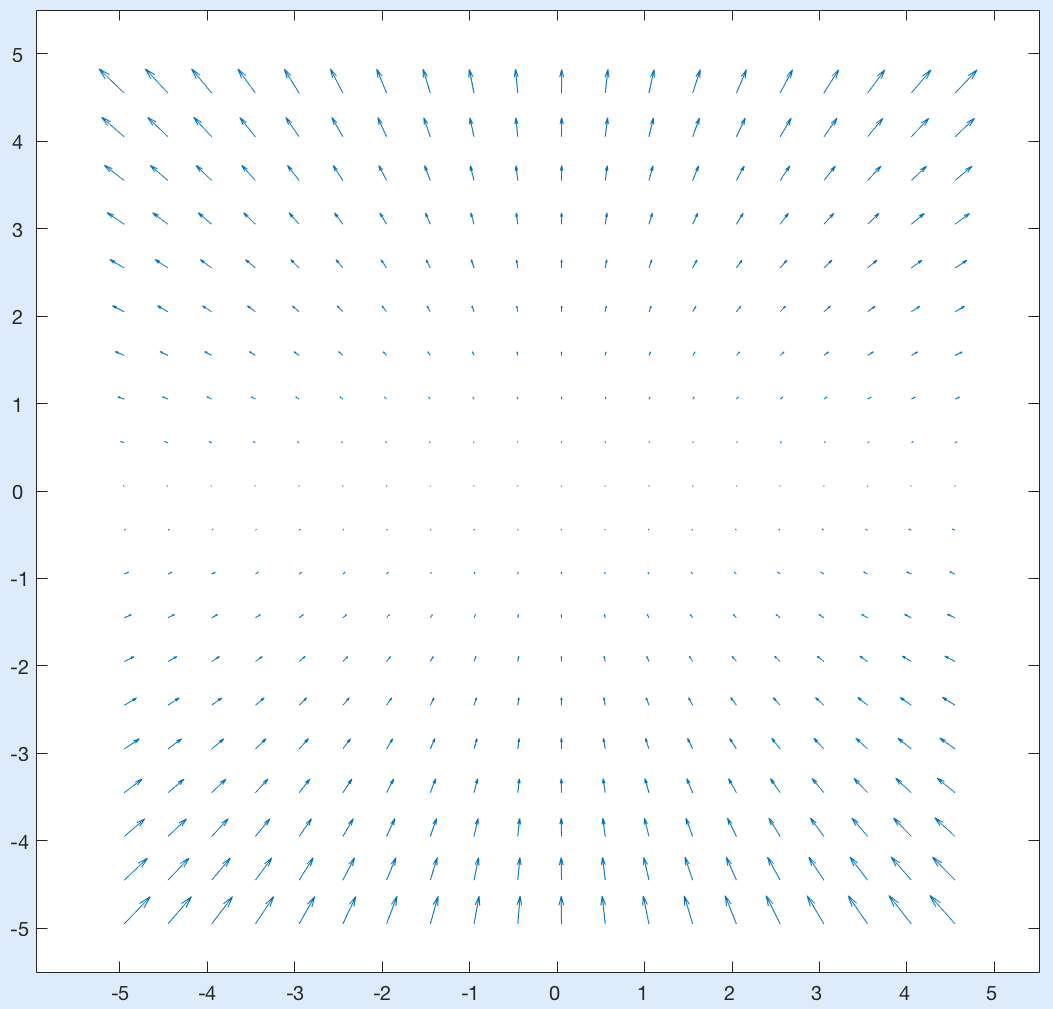
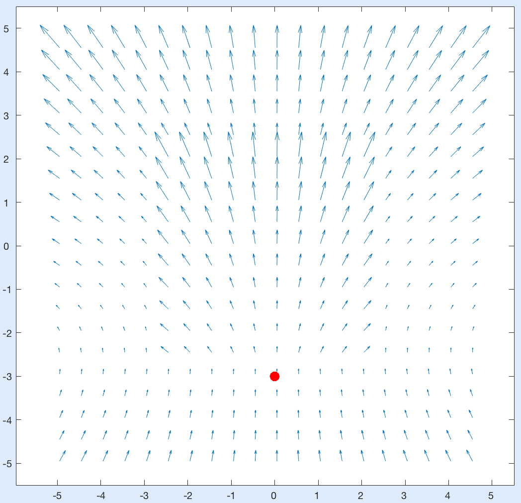
When an observer translates toward a scene without rotating their eyes or head, the velocities of features in the image are all directed away from a single location in the image that corresponds to the observer's heading point, also known as the focus of expansion, or FOE. The lines that emanate away from the FOE are sometimes refered to as the translational field lines. In this simple scenario, the speed of motion of image features depends on their location in the image and also depends on the depth of the corresponding surface points in space — the projections of more distant points move more slowly in the image. In contrast, when the observer just rotates relative to a scene without translating, the resulting velocities of image features only depend on location in the image and do not depend on depth. This is shown in the two images below. On the left is an image velocity field generated from an observer moving toward the red dot that corresponds to the FOE. The scene has a central square surface that is closer to the observer, giving rise to higher speeds in the central region of the image. On the right is a velocity field generated from an observer rotating their eyes downward while viewing the same scene — here, there is no variation in speed of motion with the depth of the viewed surface.
![]()
When the observer undergoes both motions at once, i.e. rotates their eyes as they translate toward a point in the scene, the resulting velocity field is the sum of the two fields that arise from their translation and rotation alone, as shown on the left below — this velocity field is the sum of the two fields shown above. The velocities no longer emanate from the observer's heading point.
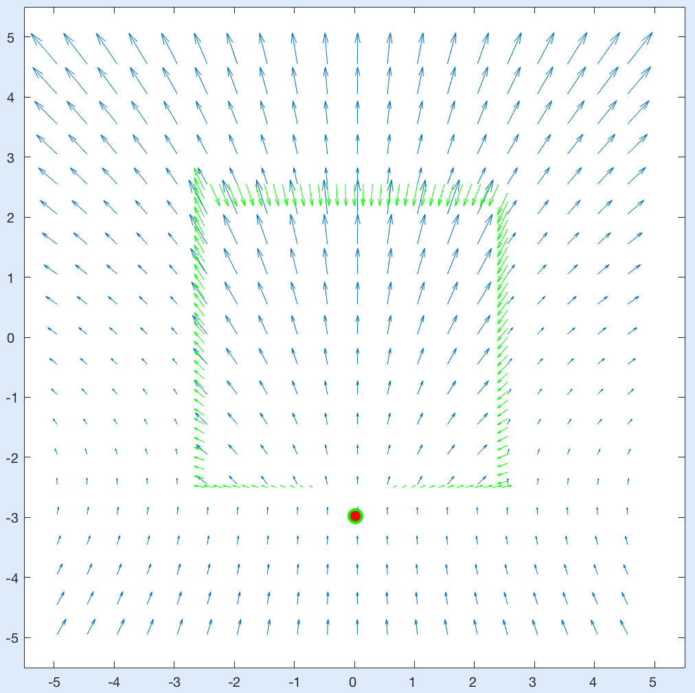
The key idea behind the Longuet-Higgins and Prazdny algorithm is that in the combined velocity field, there are still large changes in velocity across object boundaries where there is a large change in depth in the scene. In the example shown above on the left, for example, there are large changes in velocity around the borders of the central square. These changes only depend on the translation of the observer and can be used to compute the observer's heading point. To create the figure shown above on the right, the difference in velocity was computed between adjacent locations in the image, and locations of large differences were recorded. The green vectors superimposed on the velocity field show all the large velocity changes that were found, which lie along the border of the central square object. The directions of these vector differences lie along lines that roughly intersect at the observer's true heading point (the translational field lines described above). The Longuet-Higgins and Prazdny algorithm combines the directions of large velocity differences by finding the image location that best captures the intersection between these directions. For the example above on the right, this intersection point is shown with the green circle and correctly identifies the observer's heading point.
A limitation of this strategy for computing heading is that it assumes that the observer is moving relative to a stationary scene. If an object in the scene is undergoing its own motion, the changes in velocity across its borders may no longer be directed along lines that intersect at the observer's heading point. As a result, in the situation where objects move in the scene, this algorithm may yield an incorrect heading point. In this problem, you will explore a possible modification of the algorithm to detect moving objects and "remove" these objects from the heading computation. The idea is captured in steps (3) and (4) below:
- compute the velocity differences between adjacent locations in the image
- use large changes in velocity to compute an initial estimate of heading
- detect potential locations of boundary points of self-moving objects by finding locations of large velocity differences whose direction deviates significantly from the translational field lines implied by the estimated heading point in step (2)
- compute a new estimate of heading, removing the velocity differences that may come from moving objects, detected in step (3)
In this problem, you will complete the implementation of a function named detectMovingObjects
that performs step (3) in the above strategy. Skeleton code for this function is provided in the
Assign4 folder, which includes comments describing the code steps
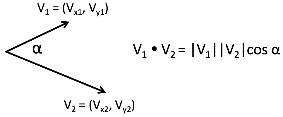
that you should complete. The figures below provide some tips related to these steps. On
the left, two vectors are shown with the angle between them labeled as α. This angle can be
calculated using the equation for the dot product of the two vectors given next to the diagram. The
MATLAB function
acosd implements the inverse cosine function and returns the angle in degrees.
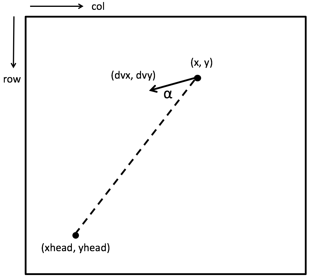
The figure on the right shows the heading point whose coordinates are given as inputs xhead
and yhead to the
detectMovingObjects function. These coordinates range from -5 to +5. The velocity
difference vector at a particular location (x,y) in the image is denoted by
(dvx,dvy) in the figure. In the code, the components of this vector are stored in two
matrices named dvx and dvy. The variables row and col,
already defined in the function, can be used to index particular locations in the dvx
and dvy matrices. Given particular values for row and col,
the simulated x and y coordinates are given by
xycoords(row) and xycoords(col), respectively, where xycoords
is a vector of coordinates ranging from -5 to +5. If the angle α computed from the velocity
difference at a particular location is too large, then this location should be labeled as a potential
boundary point of a moving object.
The objectMotionScript.m code file can be run to test your detectMovingObjects
function. It creates a scene with several rectangular surfaces at different depths and then generates
an image velocity field for an observer translating toward this scene. One object in the scene also
undergoes its own motion. The script computes an initial estimate of the observer's heading point
that is incorrect. To improve the estimation, the script performs the four steps listed above,
calling your detectMovingObjects function to determine the potential locations of
boundaries of self-moving objects, and omitting the velocity differences at these locations when
computing a new estimate of the observer's heading. The outline of the moving object is displayed at
the end.
After completing the code, answer the following questions:
- Which object is undergoing its own motion in the scene (you can just describe its location in words)?
- Given the observer's translation simulated here, is there a direction
that this object could
move that would result in the object not being "detected" by the strategy implemented in your
detectMovingObjectsfunction? - Suppose a large portion of the scene consists of objects undergoing their own motions — do you think the strategy used here would still be able to recover the user's heading? Why or why not?
- In class, we briefly summarized strategies for recovering the observer's rotation
(Rx,Ry,Rz)and layout of the scene,Z(x,y). In the process, we subtracted the image motions due to the observer's rotation from the original image velocity field, leaving us with the component of the velocity field that is due only to the observer's translation (as shown in the first image in this handout). How could this component of the velocity field then be used to further improve the estimate of the observer's heading?
Submission details: Hand in a hardcopy of the detectMovingObjects.m
code file and answers to the above questions.
Drop off an electronic copy of your code files by logging into the CS file server, connecting to your
Assign4 folder, and executing the following command:
submit cs332 Assign4 *.*