CS 332 Assignment 1 Due: Friday, September 25

This assignment focuses on the analysis of intensity changes in two-dimensional images. You will examine the results of processing a natural image at multiple scales and explore how the nature of early processing in human vision can lead to visual illusions. The final problem provides some practice with MATLAB.

The M-Files and images that you need for this assignment are contained in the edges, assign1 and assign1images subdirectories in the /home/cs332/download directory on the CS file server. These folders can be downloaded to your MAC or PC using Fetch or WinSCP. In MATLAB, set your Current Directory to the assign1 folder. In lab, you will learn how to set the MATLAB search path to include the edges and assign1images folders (this information is also contained in the Introduction to MATLAB document). Final submission details are given at the end of this handout.

Problem 1 (25 points): Processing a real image

In this problem, you will describe your observations of the zero-crossings obtained from the convolution of a real image with Laplacian-of-Gaussian convolution operators of different size. The yachtScript.m script in the assign1 folder contains the processing steps needed to generate and display an image and the zero-crossings. First open this script in the MATLAB Editor to see the code that will be executed. The yacht image is a 512x480 8-bit gray-level image of a sailing scene that is displayed using imtool. The image is convolved with two Laplacian-of-Gaussian operators with w = 4 and w = 8. Two representations of the zero-crossings of each convolution are computed - the first stores the slopes of the zero-crossings (in the matrices zc4 and zc8) and the second stores only their locations (in the matrices zcMap4 and zcMap8). All of the zero-crossings are preserved in the latter representation. The two zero-crossing maps are displayed superimposed on the original image, using imtool. You can execute this script by typing

    >> yachtScript;

in the Command Window (it will take some time to compute the convolutions). The three images that are displayed may initially be superimposed in the same region of the monitor and can be dragged apart with the mouse.

Examine the behavior of the zero-crossings for the two different operator sizes. How well do they match up with intensity changes that you see in the original image? How accurately do they seem to reflect the positions of the intensity changes? Are there "spurious" zero-crossings that do not seem to correspond to real edges in the original image? Describe specific examples of features in the image that are captured well by the zero-crossings, and places where the zero-crossing contours do not seem to correspond to a real edge in the image. Observe the image and the slopes of the zero-crossings side-by-side (the zc4 and zc8 matrices can be displayed using the displayImage function, with a border of 8 and 16, respectively). Do the slopes seem to be correlated with the contrast of the corresponding intensity changes in the image?

Problem 2 (25 points): The sun illusion

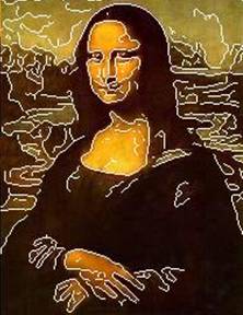
In the case of the "sun illusion" shown on the far right, we perceive a bright central disk that is not really present in the image. Occasionally one can offer a possible explanation for why these illusory contours arise, on the basis of the nature of the early processing of intensity changes that takes place in the visual system. In this problem, you will examine the zero-crossings that result from the convolution of the sun image with Laplacian-of-Gaussian operators of different size, in search for such an explanation.

The makeSun function creates an image of the sun illusion. The sunScript.m file provides some initial code for analyzing the sun image. This code convolves the image with a Laplacian-of-Gaussian operator of size w = 5 and computes the zero-crossings. The image and zero-crossings are both displayed using imtool. At this scale, the zero-crossing contours surround each spoke of the sun wheel. Add code to the sunScript.m code file to generate zero-crossings from convolutions with larger Laplacian-of-Gaussian operators of size w = 10 and w = 20. Observe the zero-crossing contours obtained from all three operator sizes and describe how they change as the operator size is increased. Based on this analysis, can you offer an explanation for the sun illusion?

Problem 3 (25 points): The Hermann Grid illusion

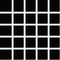
The function makeHermann creates an image of a famous contrast illusion known as the Hermann Grid. While reading a book on sound by John Tyndall in 1869 that contained a grid of bright lines on a black background, Hermann noticed that dark shadowy dots appeared at the intersections of the bright horizontal and vertical lines. You can see these dark spots in the Hermann Grid image shown below - you can see the dots more clearly at intersections that are located a small distance away from where you are directly looking. Hermann reported his observations in 1870, and since this time, the so-called Hermann Grid illusion has been much studied and debated by vision scientists. In this problem, you will explore a possible account of this phenomenon based on an analysis of the computed contrast of intensity edges (i.e. the slopes of the zero-crossings).

The hermannScript.m script file contains code for processing the Hermann Grid image by convolving it with a Laplacian-of-Gaussian operator of size w = 6 and computing the resulting zero-crossings. The image, convolution and zero-crossings are displayed using imtool. Again, they may initially be superimposed when the script is executed and can be dragged apart with the mouse. Using the Pixel Region tool in the Image Tool window, examine the slopes of the zero-crossings computed in the vicinity of an intersection of the grid, and along the middle of a horizontal or vertical bar of the grid. These two locations are indicated in the diagram below. The slope of a zero-crossing is roughly proportional to the contrast of the corresponding intensity change in the image.

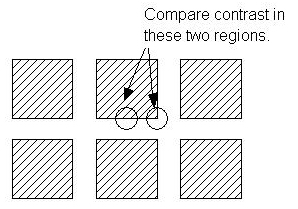
Explain why the slopes are different in the vicinity of the grid intersections and along the edges of the bars between the intersections. To assist you in answering this question, the following diagram shows the placement of the convolution operator when computing the convolution values in these two regions:

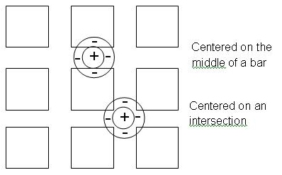
How would you EXPECT the convolution values to differ in these two areas, given your understanding of the structure of the convolution operator and the convolution computation? (Keep in mind that the intensity values for the dark regions are smaller than those for the bright bars. For both of the operator positions that are shown in the above picture, the central positive region of the operator covers an area of constant bright intensity, but the surrounding negative regions cover different amounts of dark area in the image.) The answer to this question should then lead you to an explanation of why the slope of the zero-crossings is different in these two regions. Assuming that the slopes of the zero-crossings convey information about the contrasts of the intensity changes in the original image, try to construct a possible explanation for why the intersections of the Hermann Grid appear darker. You can assume that the black regions will appear uniformly black to the human viewer.

Problem 4 (25 points): Counting cells

This problem provides some practice with writing a MATLAB script and function to analyze an image of red blood cells. The image was downloaded from the University of Virginia Health System website, http://www.healthsystem.virginia.edu/internet/hematology/hessidb/. A slightly modified version of the image, shown below, is contained in the assign1images folder, in the file cells.jpg:

Your goal is to compute a rough estimate of the number of cells in the image. Fortunately, the cells are all darker than the background and fairly well separated from one another. If you can determine the approximate number of pixels covered by a typical cell, you can then estimate the number of cells by counting the total number of dark pixels in the image and dividing this quantity by the number of pixels in a single cell.

To begin, open an empty editor window to store your script. Name the script file countCells.m and save it in your assign1 folder. The script should first load the color image cells.jpg, convert it to a gray-level image using the MATLAB rgb2gray function, and display the resulting gray-level image. Use the MATLAB help system to learn how to use rgb2gray, by executing one of the following statements in the Command Window:

    >> help rgb2gray
    >> doc rgb2gray

Your next step is to create a binary image that is a 2D matrix of values 0 and 1, where a 1 is stored at locations where the cells image contains a dark intensity value and a 0 is stored at locations of bright intensities. The following is an example of what your binary image might look like. The 1's are displayed as white and 0's are black:

To complete this step, write a MATLAB function named makeBinary that can create a binary representation of any image. This function should have two inputs: an image and number that represents a threshold value. The function should have a single output that is a 2D matrix of the same size as the input image. The output matrix should contain a 1 at locations where the input image has an intensity that is less than the input threshold, and a 0 at all other locations. The output can be a matrix of double type values. Save this function in a file named makeBinary.m in your assign1 folder.

To guide your development of the makeBinary function, consider the function findEdges that uses a simple strategy to locate intensity changes in an image:

function result = findEdges (image)
% returns a 2D matrix that is the same size as the input image,
% which contains a 1 at locations where the intensity in the input
% image differs from the intensity of a neighboring location to the
% left or above. The value 0 appears in the remaining locations.
[rows cols] = size(image);      % dimensions of the input image
result = zeros(rows,cols);      % create initial result matrix
for row = 2:rows                % loop through the rows and columns
    for col = 2:cols
        % if the intensity at this location differs from the
        % intensity of one of the neighbors, store a 1 in result
        if ((image(row,col) ~= image(row-1,col)) || ...
                (image(row,col) ~= image(row,col-1)))
            result(row,col) = 1;
        end
    end
end
imshow(result, [0 1])     % display result

There are shortcuts in MATLAB that can be used to write makeBinary with a single line of code in the body of the function, but to get practice with more MATLAB, write code that loops through the input image and compares the intensity at each location to the input threshold. Display the resulting matrix at the end of the makeBinary function.

In the Command Window, call your makeBinary function directly with the cells image and various thresholds as input, to find a good threshold that gives a result similar to the one displayed above. To guide your exploration, display the cells image with imtool and click on the blue "i" icon along the menu bar of the imtool window - an information box appears that lists the minimum and maximum intensity values in the image. You can also use the Pixel Region tool to examine the intensity values. When you find a suitable threshold, add statements to the countCells.m script that create a binary image using makeBinary and display this image in a new figure window.

Your final steps are to estimate (1) the number of pixels covered by all the blood cells in the image, (2) the number of pixels in a single, isolated cell, and finally, (3) the number of cells in the image, using the strategy described earlier. Given the binary representation of the cells image, how can you determine the total number of pixels corresponding to cells? To estimate the number of pixels in a single, isolated cell, create a copy of a small region of the binary image that includes a single, isolated cell. You can create a copy of a region of an image as shown in the following example:

    >> patch = image(30:60,40:80);