CS 332 Assignment 2 Supplement Due: Thursday, September 17

This handout provides an additional problem for Assignment 2 related to the concept of border ownership described in the article by Williford & von der Heydt.

Problem 5 (20 points): Border Ownership

In Problem 2 of Assignment 2, you explored the implementation of a region-based stereo matching algorithm, which computes a map of the stereo disparities at each location of the left image of a stereo image pair. In the resulting disparity map, a significant change in disparity signals the presence of an object boundary in the scene, which is "owned" by the surface in front. In this problem, you will implement a function that takes an input stereo disparity map and returns a matrix that encodes the side of border ownership along contours that mark significant changes in stereo disparity.

To begin, download the dispMap zip file, unzip the file, and drag the dispMap.mat file into the stereo folder that you downloaded earlier for Problem 2. A .mat file can be loaded into MATLAB with the load command:

load dispMap.mat

This file contains a single variable named dispMap that is a slightly cleaned-up version of the disparity map produced by processing the stereo images of the scene of eclectic objects that you analyzed in Problem 2. The left image and disparity map are shown below:

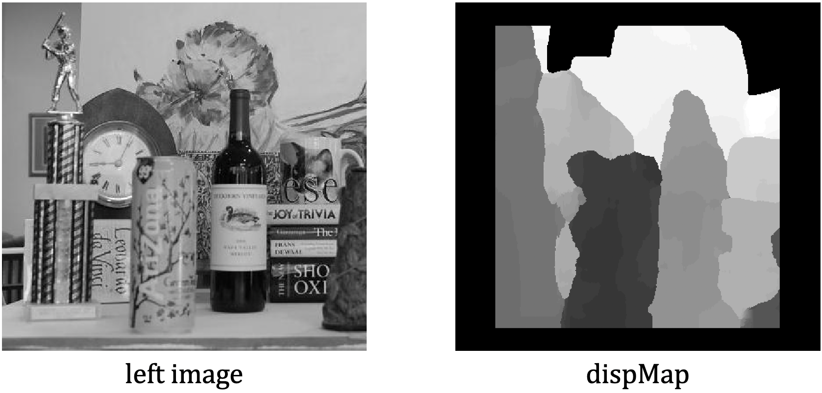
The disparity map contains disparity values that range from -16 (the front-most surface of the Arizona can) to +17 (the back wall). In the above visualization, the front surfaces (closest to the camera) are shown with darker grays and the back surfaces (furthest away from the camera) are shown as white. Along the border of the dispMap matrix, and in two areas at the top of the back wall, there are locations where disparity values were not computed. In the case of the two areas at the top of the back wall, no disparity values were computed because the average contrast in the image was too low to obtain a reliable stereo match. In locations of the dispMap matrix where no disparity is computed, the value -25 is stored (outside the range of valid disparities), which is displayed as black in the visualization above.

Define a function named borders with three inputs and one output:

function ownership = borders (dmap, nodisp, threshold)

dmap is the input disparity map and nodisp is the value that is stored in the disparity map that indicates locations where no valid disparity value was computed (-25 in this example). The input threshold is the size of the change in disparity that will be considered a significant change (a threshold value of 2 works well). This new function should be placed inside your stereo folder.

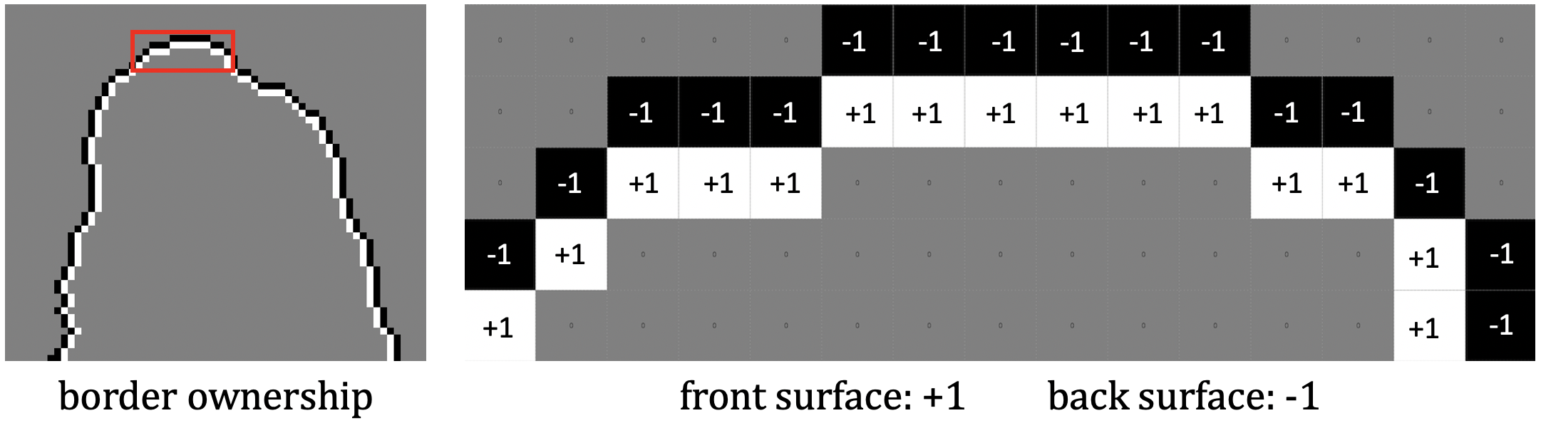
For each location of the input disparity map, the borders function should check whether there is a significant change in disparity (above the input threshold) from its two neighbors to the left or above, and if so, store values in the output ownership matrix that encode the location of the front and back surfaces at this location. The front and back surfaces can be encoded with the values +1 and -1, respectively. The figure below on the left, displays a small region of the result around the top of the wine bottle in the scene. The white pixels indicate locations of the front surface (which "owns" the border), just inside the border, and black pixels indicate locations of the back surface, just outside the border. On the right, the region highlighted with the red rectangle is shown enlarged, with the values of +1 and -1 indicating the front and back surfaces around the border:

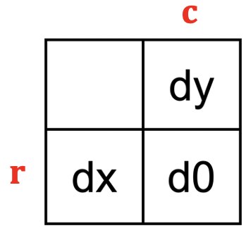
To compute the border ownership encoding, visit each location of the input disparity map. Let r and c denote the row and column of the location currently under consideration. At each location, examine the disparities stored at the current location (r,c) and its neighbors to the left and above, labeled d0, dx, and dy in the diagram below:

First check that none of the three disparity values are the input nodisp value in the function header, which indicates that no disparity was computed at the particular location. If all three locations contain a valid disparity, then examine the pair of values d0 and dx. If there is a significant change in disparity (above the input threshold), then store +1 at the location of the front surface and -1 at the location of the back surface. Then consider the current location and its neighbor above and apply the same logic. The top row of the figure below shows four examples of disparity values at a location (r,c) (circled in red in the first example) and neighboring locations to the left and above. Below each example are the resulting values that should be placed in the ownership matrix, which encode which locations are on the front and back surfaces:

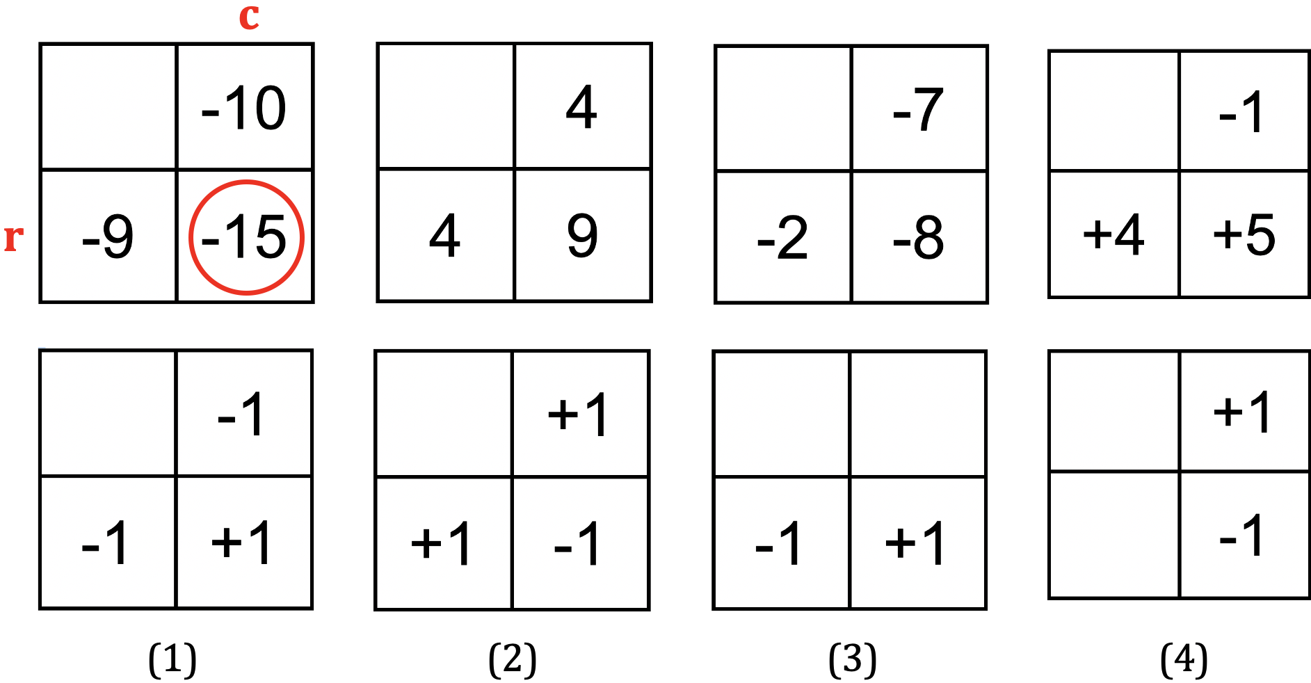
In example (1), the current location (r,c) has a disparity that is significantly in front of both neighbors, i.e. the difference in disparity is larger than the input threshold (a threshold of 2 in this case) and a disparity of -15 corresponds to a surface further in front than surfaces with a disparity of -9 or -10. In example (2), the current location has a disparity indicating that it is behind both neighbors. In the last two examples, the disparity at the current location is either in front (example (3)) or behind (example (4)) only one of its neighbors.

The following three statements load the disparity map, call the borders function, and display the results:

load dispMap.mat
ownership = borders(dispMap, -25, 2);
imtool(ownership, [-1 1])