Assignment 3
Due: Thursday, September 29
|
|
CS 332
Assignment 3 Due: Thursday, September 29 |
|
This assignment focuses on the Marr-Poggio cooperative stereo algorithm for solving the stereo
correspondence problem, and includes a problem on the recovery of depth from stereo disparity.
The M-Files that you need are contained in the stereo and
edges subdirectories in the /home/cs332/download/ directory on the CS
file server. After downloading these folders, set the Current Directory
in MATLAB to the stereo folder. When you are also using functions from the
edges folder, set the MATLAB search path
to include this folder. You will be making minor modifications to one of the code files in the
stereo folder, so you may want to store a copy of this folder on your personal directory
on the CS file server. Submission details are given at the end of this assignment handout.
In lab, you will learn how the so-called magic-eye stereograms are created. The
function magicEye in the stereo folder can
create simple color stereograms of this sort. This function has a single input that is
a matrix of disparity values, and returns an image of the same size that places randomly
selected colors at regularly spaced intervals as specified by the disparity map. The
following code segment illustrates the creation of a simple magic-eye stereogram:
>> dmap = 7*ones(200,200);

>> dmap(60:140,:) = 13;

>> magic = magicEye(dmap);
>> imshow(magic)
Examine the code for the magicEye function to see how it reflects the
basic design strategy described in lab. Try creating your own magic-eye stereogram
by modifying the construction of the dmap matrix.
Run the current script stored in the stereoScript.m code file. The script commands first
create a 50% random-dot stereogram with a pattern of disparity that consists of four concentric
circles at four different disparities (positive disparities of 0, 1, 2 and 3 pixels). The stereogram
is then displayed in two ways using the showStereogram and imshow functions.
In one window, the left and right images are shown side-by-side as black and white images. In a
separate window, the stereogram is displayed as a color anaglyph. The script then runs five iterations
of the cooperative stereo algorithm on this input stereogram, using the coopStereo
function. As the
algorithm progresses, the state of the network for each iteration is displayed in a separate window
using the showDispPlanes function. This function displays the multiple 2-D planes of the 3-D
cooperative network as separate images within a single window. The final state of the 3-D network is
displayed as a gray-level image. The various windows can be dragged apart when the script is complete.
Observe how the cooperative algorithm settles down to a final solution after only a few iterations.
Important note: After completing a run of the cooperative stereo algorithm, close the current windows and clear the current variables before running the algorithm again:
>> close all

>> clear all
Also note that when MATLAB is busy executing code, the word Busy appears near the
bottom left corner of the MATLAB window.
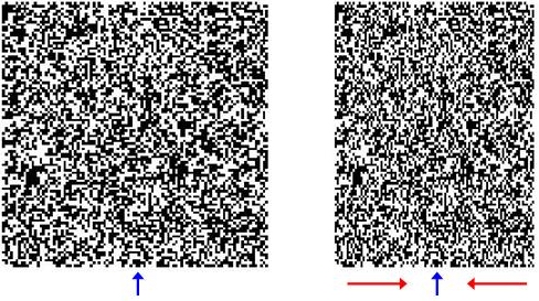
Suppose we create a random-dot stereogram that has zero disparity everywhere (i.e. the left and right images are identical) and then condense the right image uniformly in the horizontal direction, as suggested by the red arrows in the figure below. Based on your understanding of the geometry of the projection of points in space onto the left and right eyes, what would you expect observers to see when viewing this stereogram? Explain your answer using geometric arguments. For simplicity, you can assume that the central column of the left and right images projects to the same position in the left and right eyes, so that it has zero disparity, as suggested by the two blue arrows in the figure.
One of the constraints used in the cooperative stereo algorithm is the uniqueness constraint -
this constraint is based on the assumption that each feature in the left image should match a single
feature in the right image. In this problem, you will explore the performance of the algorithm on a
random-dot stereogram that violates the uniqueness constraint. This stereogram has 10% white dots and
90% black dots in the left image. To create the right image, each white dot in the left image was copied
twice in the right image, at two different disparities of 0 and 4 pixels. Stereograms like this are
sometimes referred to as Panum's limiting case in the literature. In the
stereoScript.m code file, comment out the statements from the first example and uncomment the
statements that create and display this stereogram,
which is constructed with the makeDoubleStereogram function. View this stereogram as a color
anaglyph and describe in words, what you perceive. Make one or more predictions about how the cooperative
stereo algorithm might perform on this stereogram. Do you think it will eventually compute a single
disparity for each dot in the left image? Do you think the two different disparities will be evident in
the final solution? After making your prediction(s), run the cooperative algorithm (uncomment the
statements that call the coopStereo function on this stereogram and display the results)
and observe its behavior. How would you characterize the final solution reached by the cooperative stereo
algorithm? How does it compare to your prediction(s)? Does the final solution violate the uniqueness
constraint?
In this problem, you will examine in more detail, how the cooperative stereo algorithm behaves on a
sparse random-dot stereogram. In the stereoScript.m code file, uncomment the statements
that create a sparse stereogram from the concentric-circles disparity map. This stereogram has only
10% white dots and 90% black dots in both the left and right images. If you run the cooperative stereo
algorithm on this 10% random-dot stereogram (the commands for this are also given in the script file)
and compare the results to those obtained for the 50% random-dot stereogram, you will observe that
the stereogram with the lower density of white dots requires more iterations to converge to a stable
solution, and the final solution does not have the clean, smooth edges around the concentric circles
that appear in the results obtained for the denser stereogram. Why are more
iterations required to compute the disparities of points in the stereogram with lower dot density?
Why are the outlines of the concentric circles so rough? Hints: consider the difference
between the initial states of the network for the two stereograms - for the 10% random-dot stereogram,
how would you expect the initial states for the black and white dots to differ? Consider how the
algorithm tries to compute a single disparity for each location, and how the disparity information at
one location spreads to other locations nearby.
Suppose you construct a stereogram with a small object at one constant disparity, surrounded by a
background that has a different constant disparity. How small can this object be, and still "survive"
the stereo matching process? At some point, the desire of the cooperative algorithm to impose the
constraint of continuity will result in a smoothing of the computed disparities across the object, and
the object will not be preserved in the final disparity map (i.e. after some number of iterations, the
surrounding disparity will spread through the object). To explore this question, you can work with a
stereogram that contains one or more small patches at different disparities from the background. As a
starting point, the stereoScript.m file contains statements that create and display a
stereogram from a disparity map that has four different square patches whose sizes are 16, 8, 4 and 2
pixels on a side. The disparity of each patch is 4 and the background disparity is 0. First run the
cooperative stereo algorithm on this example to see which of the patches survive the matching process.
Note that you may need to watch the behavior of the algorithm over a larger number of iterations to be
sure that the patch really survives. Modify the patch sizes created in the dmapPatches
matrix and run the stereo algorithm again, to determine what is the smallest size patch that survives
the matching process. Describe your observations and explain why very small patches of
different disparity can "disappear" in this way.
The minimum size of patch that survives depends on the values of the parameters epsilon and
threshold in the middle of the coopStereo function.
Choose one of these
parameters and observe the change in the behavior of the algorithm (in particular, the size of the
minimum patch that survives may change). Try to explain why the behavior is different. In the case of
epsilon, the default value is 2.0 and you might try values such as 1.0 and 3.0. The default
value of threshold is 3.0, and here you might try values of 1.0 and 5.0 as a start.
After completing your simulations for this problem, be sure to change epsilon and
threshold back to their original values for other problems!
The previous problems used random-dot stereograms directly as the input to the cooperative stereo
algorithm, and used the dots themselves as the features that are matched between the left and right
images. In this problem, you will use the zero-crossings of the result of convolving an image with a
Laplacian-of-Gaussian operator as the matching features. The detection and description of the
zero-crossings for stereo matching differs from the strategy used previously in the zeros2D
function, however, in the following ways. First, horizontal
segments of the zero-crossing contours are not used in the stereo matching process, because the
relative positions of points along horizontal contours is ambiguous. Second, the magnitude of the
slope of the zero-crossing is not considered for the stereo matching process - only the sign of
the zero-crossing is represented. In particular, if the convolution is increasing from left to right
at the location of a zero-crossing (a positive zero-crossing), the value 1 is placed in the
resulting zero-crossing matrix. If the convolution is decreasing from left to right at the location
of a zero-crossing (a negative zero-crossing), the value -1 is placed in the resulting
zero-crossing matrix. The value 0 is placed in locations that do not correspond to a zero-crossing.
The zero-crossings for stereo processing are computed by the stereoZeros function in
the stereo folder.
Uncomment the statements at the beginning of stereoScript.m that create dmapCake,
leftC, and rightC (the 50% random-dot stereogram with concentric circles of different
disparity), and statements at the end of the script that compute the
convolution of the leftC and rightC images
with a Laplacian-of-Gaussian operator and call the stereoZeros function to
compute the zero-crossings of the two convolutions. Further statements display the two zero-crossing
patterns (stored in the zcLeft and zcRight matrices) side-by-side, using
imshow. In the resulting display, positive zero-crossings appear as white points,
negative zero-crossings appear as black points, and the background is gray. Finally, uncomment the
statements that run the cooperative stereo algorithm on this stereogram and display the final
results.
Compare the behavior of the stereo algorithm when the stereogram itself is used to construct the initial state, to the behavior observed when the zero-crossings are used to construct the initial state. How does the appearance of the initial state differ? How many iterations are needed in both cases for the algorithm to converge to a stable solution? How does the final solution differ? Why does the behavior differ? Hint: Consider your answers to Problem 3, in which you analyzed the behavior of the algorithm on a sparse random-dot stereogram.
Submission details: Hand in a hardcopy of your answers to these problems. There is no need to hand in electronic copies of any files.