CS 332 Assignment 4 Part 1 Due: Friday, November 5

This first problem for Assignment 4 explores the performance of the Eigenfaces method for recognizing faces, which is based on Principal Component Analysis (PCA). The code and image files for this problem are stored in a folder named eigenfaces that can be downloaded through this eigenfaces zip link. (This link is also posted on the course schedule page and the eigenfaces folder is also stored in the /home/cs332/download directory on the CS file server.)

Submission details: For this problem, create a shared Google doc with your partners (be sure to add all your names to the top of the document). You can then submit this work by sharing the Google doc with me — please give me Edit privileges so that I can provide feedback directly in the Google doc.

Problem 1: Eigenfaces for Recognition

In this problem, you will explore the behavior of the Eigenfaces approach to face recognition proposed by Turk and Pentland, which is based on Principal Component Analysis (PCA). You do not need to write any code for this problem — you will explore the method with a GUI based program that a previous CS332 student, Isabel D'Alessandro '18, helped to create. To begin, set the Current Folder in MATLAB to the eigenfaces folder. To run the GUI program, enter facesGUI in the MATLAB Command Window. When you are done, click on the close button on the GUI display to terminate the program. 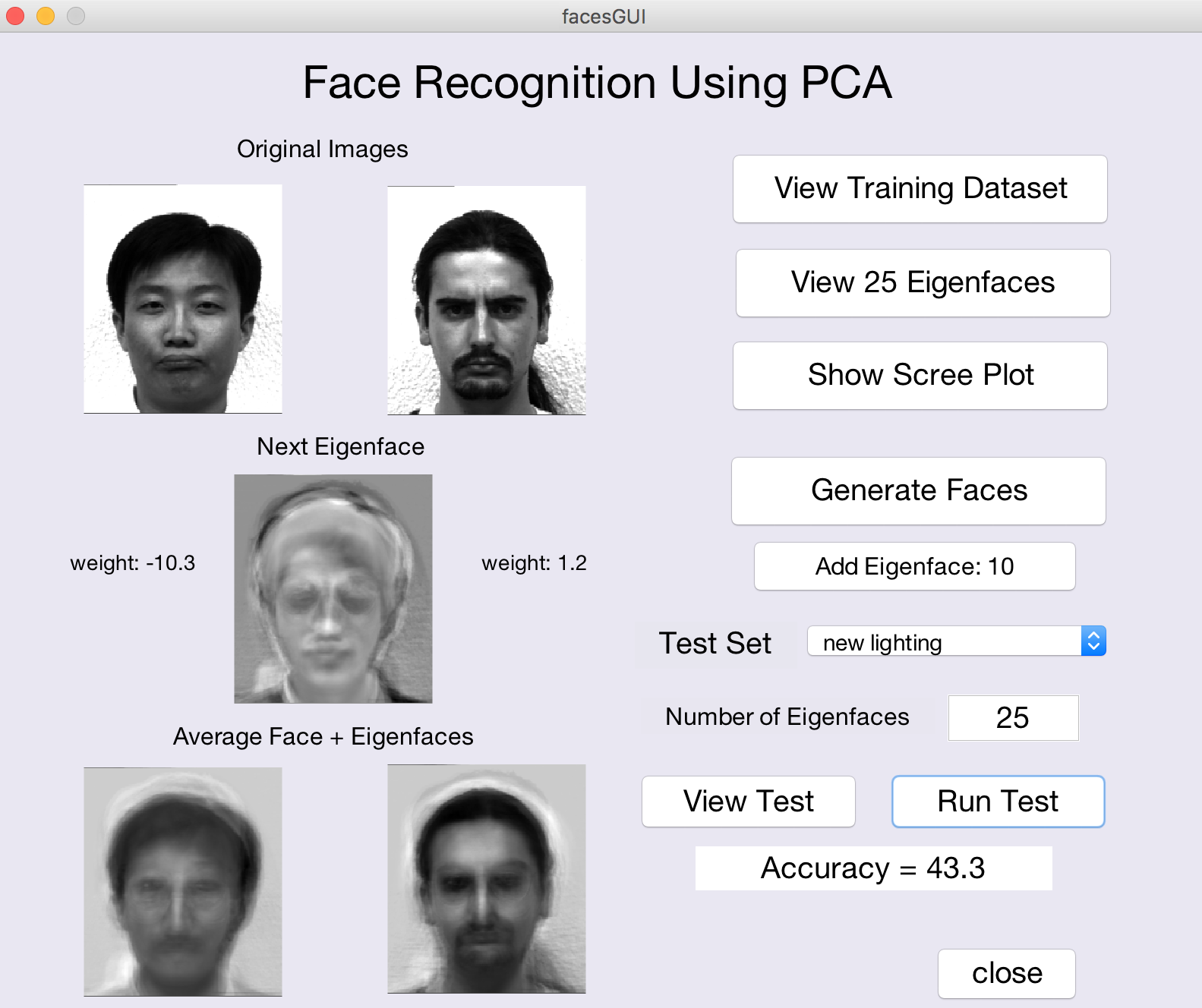The figure below shows a snapshot of the program in action:

            

The program uses an early version of the Yale Face Database that consists of 165 grayscale images (in GIF format) of 15 different people (I'm sorry there is only one woman in the database!). There are 11 images per person, taken under different conditions (central light source or lighting from the left or right; neutral, sad, happy, and surprised expressions; with and without glasses; sleepy and winking). I created two additional images of each person by rotating the neutral-expression images by 15 degrees in the clockwise and counterclockwise directions.

A subset of 7 images for each of the 15 people (omitting the left/right lighting conditions, happy/surprised emotions, and rotated images) is used as the training set to compute the eigenfaces (principal components) that capture the variation across this dataset of face images.

• View the full training set by clicking on the View Training Dataset button.
• Click on the View 25 Eigenfaces button to see the top 25 principal components. The first principal component, which captures the largest variation in the data, is shown in the upper left corner, and components that capture progressively less variation (e.g. eigenvectors with smaller eigenvalues) are displayed from left to right within each row, and then from top to bottom. Select two of the eigenfaces and describe in general terms, what features of a face image may be altered if a very large or very small (positive or negative) weight were associated with each of these two eigenfaces.
• Click on the Show Scree Plot button to see a scree plot in which the eigenvalues associated with the principal components are displayed as a function of the component number (in decreasing order). The scree plot can be used to assess visually, how many components need to be preserved in order to explain most of the variability in the data. This is shown more directly in the bottom graph that plots the cumulative amount of variation in the data that can be explained as more principal components are considered. How many components are needed to explain at least 90% of the variance of the data?

In class, we showed how an image can be expressed as the sum of an average face and a weighted sum of a subset of the eigenfaces. If you click the Generate Faces button, two randomly selected images from the training set will be displayed in the upper left corner of the GUI. The average face computed from the full training set is shown in the two display areas at the bottom of the GUI window. In the center, you will see the first eigenface, with the weights associated with this eigenface, obtained for the two face images shown. The Add Eigenface button will be enabled, allowing you to incrementally add each eigenface (with associated weights) to the average faces at the bottom, using the individual weights for each of the two face images. As you continue to click on the Add Eigenface button, you will see the two individual identities emerge.

• For a few different pairs of images, observe the evolution of the composite image as more eigenfaces are added, and the different weights for each eigenface associated with each of the two face images (you do not need to record this information, just make a mental note). How many eigenfaces does it typically take to start distinguishing the two faces? How many eigenfaces are typically needed to create an identifiable version of each face?

Once the eigenfaces, or principal components, are computed, we can then try to recognize the person depicted in a novel image, and examine how the representation generalizes to handle, for example, different lighting, expressions, and orientations of a face. Using the popup menu to the right of the Test Set label, you can select one of three different test sets. View the face images that comprise each test set by making a selection and then clicking the View Test button (you will see a skinny window with two columns of face images). If you click on the Run Test button, the percentage of the test images that are correctly identified will be printed in the text box below this button. You can also modify the number of eigenfaces that are used to represent each of the training and test images. Based on the accuracy results obtained for different choices of test set and number of eigenfaces used, answer the final questions below.

• How well does the method generalize to different lighting conditions? to different emotions? How well does it tolerate small rotations in the image? How do the results depend on the number of eigenfaces used? Over what range do you see improvement in the results (this may vary for the different test sets). Why might you expect to obtain the results that you did? Relate the results to the nature of the information used by the PCA method to perform recognition.