Assignment 6
Part I
Due: Wednesday,
November 11
|
|
CS 332
Assignment 6
Due: Wednesday, |
|
This first part of Assignment 6 contains one problem related to the recovery
of the motion of an observer from 2-D image velocities. To begin this problem,
first download the following folder from the CS file server:
/home/cs332/download/observer and set the Current Directory in
MATLAB to this folder.
Part a: The following equations specify the x and
y components of the image velocity (Vx,Vy)
as a function of the movement of the observer (translation
(Tx,Ty,Tz) and rotation
(Rx,Ry,Rz)) and depth
Z(x,y):
Vx = (-Tx + xTz)/Z + Rxxy -
Ry(x2+1) + Rzy
Vy = (-Ty + yTz)/Z +
Rx(y2 + 1) - Ryxy - Rzx
Write a function setupImageVelocities that computes the image velocity
field that results from a movement of the observer:
function [vx vy xfoe yfoe] = setupImageVelocities(Tx,Ty,Tz,Rx,Ry,Rz,zmap)
The input zmap is a 2-D matrix of the depths of the surfaces that project
to each image location. The output matrices vx and vy should
be the same size as the input zmap. Assume that the origin of the
x,y image coordinate system is represented at the center of the
zmap, vx and vy matrices. The indices of these matrices should
also be scaled to obtain the x and y coordinates that are
used in the above equations. In particular, let i and j
represent the indices of the zmap, vx and vy matrices
(where i is the first index and j is the second), and
let icenter and jcenter denote the indices of the center
location in these matrices (icenter is the middle row and
jcenter is the middle column). Then the x and y
coordinates that are used in the above expressions for Vx and
Vy should be calculated as follows:
    x = 0.05*(i-icenter);

    y = 0.05*(j-jcenter);
The setupImageVelocities function should also return the x
and y coordinates of the focus of expansion,
Tx/Tz and Ty/Tz
(if Tz is 0, then this function can just return a value such
as 1000.0 for the coordinates of the focus of expansion, to indicate that it is
undefined in this case). The function displayVelocityField in the
observer folder displays velocities at evenly spaced locations in the
horizontal and vertical directions. It has three inputs that are the vx
and vy matrices and the distance between the locations where a velocity
vector is displayed. The foeScript.m code file contains some initial
statements for testing your setupImageVelocities function and displaying
the results. The depth map used in these examples consists of a central square
surface at a distance of 25 from the observer, in front of a background surface at a
distance of 50. There are three examples, and each velocity field is displayed in
a separate figure window. The coordinates of the FOE's are also printed.
You can expand on these examples to explore the appearance of the
velocity field for different combinations of translation and rotation of the
observer, and surface depths. Given the depths and image coordinates used in the
initial examples, velocities with a reasonable range of speeds can be obtained if
the translation parameters are specified in the range of about 0.0-0.5, and the
rotation parameters are specified in the range of about 0.0-0.03.
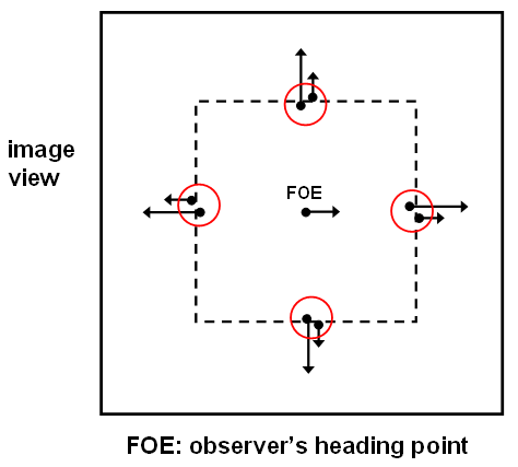
Part b: In class, we discussed an algorithm for recovering the direction
of motion of the observer that was proposed by Longuet-Higgins and Prazdny. This algorithm
is based on the following observation. At the location of a sudden change in depth in the
scene, the component of image motion due to the observer's translation changes abruptly
in the image, but there is very little change in the component of image motion that is due
to the observer's rotation. Furthermore, the vector difference between the two 2-D image
velocities on either side of a depth change lies on a line that points toward the focus of
expansion (the observer's heading point). The computeObserverMotion function
in the observer folder
implements a simple version of Longuet-Higgins and Prazdny's
algorithm. At each image location, this function first determines whether there is a large
change in 2-D velocity in the horizontal or vertical direction. If so, the vector
difference in velocity in the horizontal or vertical direction contributes toward the
computation of the observer's heading point. To determine this heading point, the function
combines velocity differences from a large number of image locations. In particular, it
finds the best intersection point of all of the lines containing large velocity
differences. There are two tests of the computeObserverMotion function in the
foeScript.m code file that are initially commented out. Each call to this
function is followed with a statement (also initially in comments) that prints the values
of the coordinates of the true heading point and the computed heading point for each
example. The true and computed values can be compared to determine the accuracy of
computed heading. Expand on the examples provided in the foeScript file to
demonstrate the following two properties:
Submission details: Hand in a hardcopy of your
setupImageVelocities.m
code file and your answers to the questions in this problem.
Please also hand in an electronic copy of the setupImageVelocities.m
code file by posting a message to the CS332-01-F09 Drop conference with
this code file as an attachment.