
|
|
Assignment 4
|
|
Due: Thursday, March 12, by 5:00pm
You can turn in your assignment up until 5:00pm on 3/12/20. You should
hand in both a hardcopy and electronic copy of your solutions. Your hardcopy
submission should include printouts of four code files:
spin.m, lineFit.m, poleVault.m, and visualize.m.
To save paper, you can cut and paste all of your code files into one file, but your
electronic submission should contain the three separate files.
Your electronic submission is described in the
section How to turn in this assignment.
If you need an extension on
this assignment, please see the Late Assignment Policy
on the Course Information Page.
This assignment contains one programming exercise and two extended problems. You will work on the exercise with a partner in your lab and should complete the exercise with that partner. You are free to choose any partner to complete the problems, including a partner from a different lab.
Reading
The following material from the fifth or sixth edition of the text is especially useful to review for this assignment: pages 187-188, 192-196, 200-202, 221-231. You should also review notes and examples from Lectures #9, 10 and 12, and Lab #5.
Getting Started: Download assign4_exercise and assign4_problems
Use Cyberduck to
connect to the CS server and download a copy of the
assign4_exercise folder onto your Desktop. This folder contains one file named rotate.m for
the exercise in this assignment. When you are ready to begin the problems, download a copy of the
assign4_problems folder onto your Desktop. This folder contains a data file for
Problem 1 named poleVaultData.mat and a data file and code file for Problem 2 named
rising_data.mat and test_visualize.m.
Uploading your completed work
When you have completed all of the work for this assignment, your
assign4_exercise folder should contain one additional file:
-
spin.m
Your assign4_problems folder should contain three code files:
-
lineFit.m -
poleVault.m -
visualize.m
Use Cyberduck to connect to the CS file server and navigate to your
cs112/drop/assign04 folder. Drag your assign4_exercise and
assign4_problems folders to this drop folder. More details about this process
can be found on the webpage on Managing Assignment Work.
Exercise: Spirograph 
In this exercise, you'll write a function called
spin.m that will spin a set of coordinates around in a
circle. You are provided with a function called rotate.m (in the
assign4_exercise folder)
that has three inputs: 1) a vector of x coordinates, 2) a vector of y
coordinates, and 3) the angle in degrees to rotate those coordinates.
First, make sure you understand how rotate works, because your
function spin will rely upon rotate. (You do not need
to make any changes to rotate.m.)
Understanding rotate.m
Let's take a concrete example of a square. A square with side length 5 can be drawn using these two vectors:
 xsquare = [3  8  8  3  3];
 ysquare = [3  3  8  8  3];
 plot (xsquare, ysquare);
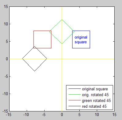
|
The following code (the code to generate the yellow axis and the "original square" text in the box is not shown here) produced the green, red and black rotated squares at left:
|
The function rotate always takes three inputs and returns
two output vectors.
Note that the examples above rotate a square, yet
rotate can rotate any set of x and y coordinates.
Writing spin.m using rotate.m
Your task is to write the function spin using
rotate. The spin function will take in three inputs: 1) a
vector of x coordinates, 2) a vector of y coordinates, and 3) the
number of times to repeat the coordinates in the design.
spin will create a design in a MATLAB figure window.
The steps below will incrementally build your spin function. You need only turn in the final
version of spin. In the examples below, the same x and y coordinates are used for the square as
above. The flower petal coordinates are as follows:
 xpetal = [0  2  8  6  0];
 ypetal = [0  4  5  2  0];
- For this first simple version,
spintakes only two inputs: the x and the y coordinate vectors. This version ofspinwill always produce 8 sets of rotated coordinates and plot them in the default blue color.

spin(xsquare, ysquare)spin(xpetal, ypetal) - Now edit your version of
spinso that there is a third input, namely, the number of rotations to be plotted. Your editedspinshould plot the user-specified number of rotations of the x and y coordinates, as in the figures below.

spin(xpetal, ypetal, 5)spin(xsquare, ysquare, 11)

spin(xsquare, ysquare, 20)spin(xpetal, ypetal, 20) - The final version of
spinproduces a user-specified number of rotations of the given x and y coordinates in multiple colors. The examples below cycle through the available colors and show 50 rotations of each set of coordinates.

spin(xsquare, ysquare, 50)spin(xpetal, ypetal, 50)
spin that you submit: the function takes three inputs
(x coordinates, y coordinates, and the number of rotations to be plotted) and produces one colorful
figure.
Problem 1: Able to leap tall buildings in a single bound!
One true test of any scientific theory is whether or not it can be used to make accurate predictions. Given some data that captures the relationship between two or more variables, we can try to formulate a mathematical model that summarizes this relationship. If the model is valid, it can be used to predict the relationship between the variables in cases not explicitly given in the original data.
In some cases, variables may have a simple linear relationship, such as in
the forearm and hand data that we used to test the existence of the Golden Ratio:
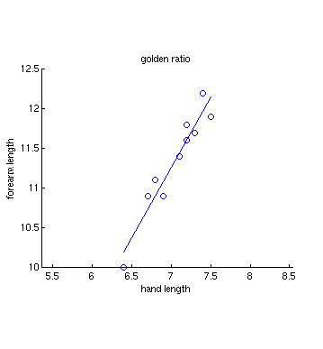
The line drawn through the points is the best fit line for the data, also
referred to as the regression line. MATLAB provides functions for fitting lines
and other curves to data, but you will instead write your own function to compute the
regression line for a set of data, and tailor the information that is returned.
You will then apply this analysis to data on the achievements
of olympic pole vaulters in the summer olympics, from 1896 to 2004. Finally, you
will analyze the pole vaulting data using the Curve Fitting Toolbox that you explored in
lab.
Computing a regression line
A nice introduction to the computation of regression lines is provided online at this Finite Mathematics & Applied Calculus resource developed by Stefan Waner and Steven Costenoble at Hofstra University.
Given the (x,y) coordinates for a set of n points (x1,y1), (x2,y2), ... (xn,yn), the best fit line associated with these points has the form
y = mx + b
where
slope m = (n(Σxy) - (Σx)(Σy)) / (n(Σx2) - (Σx)2)
intercept b = (Σy - m(Σx)) / n
The Σ means "sum of", so
Σx = sum of x coordinates = x1 +
x2 + ... + xn
Σy = sum of y coordinates = y1 +
y2 + ... + yn
Σxy = sum of xy products = x1y1 +
x2y2 + ... + xnyn
Σx2 = sum of squares of x coordinates =
x12 + x22 + ... +
xn2
When performing linear regression, it is valuable to know how well the line actually
fits the data. Two measures used to assess the quality of fit are the correlation
coefficient and the size of the residuals that capture the difference between
the actual data values and the values predicted by the regression line. The correlation
coefficient, also described in the Waner and Costenoble online chapter, is a number
r between -1 and 1 calculated as follows:
coefficient r = (n(Σxy) - (Σx)(Σy)) / [n(Σx2) - (Σx)2]0.5[n(Σy2) - (Σy)2]0.5
A better fit corresponds to a value of r whose magnitude is closer to 1,
while a worse fit yields a value of r closer to 0. The residuals are the
discrepancies between the actual data (actual y values) and those predicted by the
best fit line (the values mx + b). A rough estimate of the average size of the
residuals is given by the RMS error between these two quantities:
average residual RMS = ((Σ(y - (mx + b))2) / n)0.5
Implementing linear regression
Write a function named lineFit that has two inputs that are vectors containing
the x and y coordinates of a set of points. This function should return four values, all obtained using
the above calculations: the (1) slope m and (2) intercept b of the best fit line,
the (3) correlation coefficient and (4) average residual. Test your function with a small number
of points that you create. You can check your results for the best fit line against
those obtained with the MATLAB polyfit function, which returns a vector
containing the m and b values:
>> lineMB = polyfit(xcoords, ycoords, 1)
Note: you do not need to use any loops (for statements) in your
lineFit function - all of the calculations can be done by performing
arithmetic operations on the entire vectors of x and y coordinates all at once. This
problem primarily provides practice with writing a function with multiple inputs and
outputs, and more experience with curve fitting.
Hint: The following function illustrates the use of multiple inputs and outputs to perform simple computations on two input vectors and return the results:
function [sumV diffV prodV divV] = compute(vect1, vect2)
% [sumV diffV prodV divV] = compute(vect1, vect2)
% computes the element-by-element sum, difference, product and division
% of the values in two input vectors and returns the four results
sumV = vect1 + vect2;
diffV = vect1 - vect2;
prodV = vect1 .* vect2;
divV = vect1 ./ vect2;
The future of olympic pole vaulting
From the time the summer olympics began in 1896, until 2004, pole vaulters achieved heights
that increased in a roughly linear fashion (heights are given in inches):
|
In the assign4_problems folder, there is a MAT-file
named poleVaultData.mat
that contains two variables years and heights that store the above data.
Write a script file named poleVault.m that performs the following actions:
- loads the
poleVaultData.matfile - plots the data (height vs. year) using the
scatterfunction to create a scatter plot:scatter(xcoords, ycoords)Check the MATLAB help pages for properties that can be used to change the appearance of the dots, and incorporate some of these properties into your scatter plot.
- calculates the best fit line using your
lineFitfunction - draws the best fit line superimposed on the scatter plot, using the
plotfunction (remember that you only need two points to draw a line!) - assuming that this is an accurate model for predicting the future of pole vaulting, predict the year in which pole vaulters will be able to leap tall buildings in a single bound - in this case, Green Hall, which reaches 182 feet from the ground to the highest finial
- prints the predicted year in which a pole vaulter will leap over Green Hall - the floating
point value for this year can be converted to an integer using the
uint16function:>> uint16(5626.7864)
ans =
5627
In a comment at the end of the poleVault.m script, write the predicted
year that is printed by your script, and also comment on the reasonableness of the model.
![]()
Using the curve fitting tool
After running your poleVault.m script, the two variables years and
heights will be stored in your Workspace. Open the curve fitting tool with the
cftool function and create a data set with years as the X data and
heights as the Y data. A linear polynomial fit to this data should yield a line
similar to what you obtained with your linefit function. A better model of
pole vaulting performance, though, would use a function that reaches a plateau as
the year increases. One example is a logarithmic function. To obtain a fit to a log function,
select Custom Equation for the type of fit.
A default exponential equation will appear in the
equation box. Replace this expression with the following general logarithmic expression:
a * log(b*(x-1895))
The logarithmic function does not
fit the past data as tightly, but probably has better predictive capability for the future.
Use both the logarithmic curve fit and a linear curve fit to predict pole vaulting heights
for the year 3000. Record this information in your poleVault.m script file
and comment on which fit appears to yield a more reasonable prediction.
Problem 2: Rising Data
This problem was inspired by a visualization of rising global temperatures at the Bloomberg Company website. You will write a function to create your own visualization of rising data of this sort, and apply this function to data on rising monthly temperatures in the Boston area over the years from 1880 to 2014, and rising daily Dow Jones Industrial Averages over 51 weeks of 2014. An advantage of defining a function to create this visualization, rather than a script, is that a function can easily be applied to different data sources that are provided through an input to the function.
In the assign4_problems folder, there is a data file named rising_data.mat
that contains two variables, temps_data and djia_data. The variable
temps_data is assigned to a 135 x 12 matrix, where each row corresponds to a different year
(1880 to 2014) and each column corresponds to a different month (January through December). The values
stored in the matrix are the average monthly
temperatures in degrees Celcius. The variable djia_data is assigned to a 51 x 5 matrix,
where each row corresponds to a different week during the year 2014 and each column corresponds to a
different weekday (Monday through Friday). The
values in this matrix are the closing Dow Jones Industrial Averages for each day. The
assign4_problems file also contains a script named test_visualize that loads
the data files and calls the visualize function (that you will write) for each of these two
data sources. Your visualize function should have five inputs:
- a 2D matrix of data where the rows and columns represent different time frames (e.g. years x months or weeks x days)
- a string to display as the label of the x axis of the data plot
- a string to display as the label of the y axis of the data plot
- a string to display as the title of the plot
- a cell array of strings to display below the tick marks on the x axis
The two calls to the visualize function in the test_visualize script
provide examples of these inputs. Your function should loop through the rows of data in the input
data matrix and display one after the other on the same figure. After displaying each new plot, add
a short pause to the code inside your loop. The built-in MATLAB function pause() has a
single input that is the number of seconds to pause. For example, the statement pause(0.1) will cause
MATLAB to pause for one tenth of a second before continuing the execution of your code. The pause
will cause the presentation of the successive plots to appear as an animation,
similar to the Bloomberg visualization mentioned above. As you are looping
through the rows of data, when the average of the newly displayed data breaks a record
(i.e. the mean of the data values in the new row is higher than the mean of all previously displayed
rows), display a horizontal dotted line at the new record mean data value. Finally, each row of data
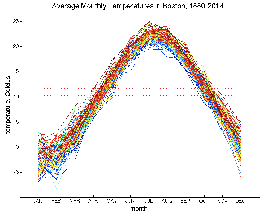
should be displayed with a different color. The
two figures below show the full sets of data that should be visible when the animation is complete. The
dotted horizontal lines show the average temperature or Dow Jones values during record breaking
years or weeks, respectively. The colors change from "cool" shades of blue to "hot" shades of red as
time progresses.

The following are a few guidelines and tips for implementing the visualize function:
- the input data matrix should be a required input, while the other four inputs should be optional; the default values for the x label, y label, and title can be an empty string or some generic string, and the default value for the tick marks on the x axis can just be the column numbers for the data matrix
- create a fairly large figure window for your graph, using the
'Position'property, e.g.figure('Position', [100 100 1000 800]); - in Assignment 2, you learned how to place string labels on the x axis tick marks, e.g.
set(gca, 'XTickLabel', {'Democrats' 'Republicans' 'Independents'})
The
'FontSize'property can also be used with thesetfunction to set the size of the font used to display the strings. This property can also be used with thexlabel, ylabelandtitlefunctions. - in advance of plotting the rows of data, determine the overall range of the data and use the
axisfunction to set appropriate ranges of values for the x and y axes, so that the axis ranges are not automatically readjusted as the animation progresses.
We have been using single characters, like 'r' and 'g', to specify the color of a plot. An arbitrary
color can be specified with a vector of three values that are each between 0 and 1 and represent the
amount of red, green, and blue that combine to create the desired color. When calling the plot
function, this color vector can be specified with the 'Color' property, e.g.
plot(xcoords, ycoords, 'Color', [0.3 0.8 0.7]);
which creates a plot with a teel blue color. MATLAB provides a set of built-in color palettes, or
colormaps, that you can view in the MATLAB documentation on the
colormap function. Each color palette
has a name and is associated with a built-in function of the same name that can be used to generate an
n x 3 matrix with red, green, and blue values for a set of n colors that span the palette. One of the
palettes, for example, is named jet and spans the colors of the rainbow from blue to red.
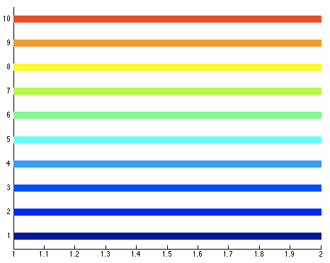
The function call jet(10) creates a 10 x 3 matrix storing 10 sample colors from blue to red:
>> colors = jet(10)
colors =

         0         0    0.6667
         0         0    1.0000
         0    0.3333    1.0000
         0    0.6667    1.0000
         0    1.0000    1.0000
    0.3333    1.0000    0.6667
    0.6667    1.0000    0.3333
    1.0000    1.0000         0
    1.0000    0.6667         0
    1.0000    0.3333         0
>>
These colors were used in a loop to create the following plot of 10 horizontal lines of different colors:
You are welcome to use any of the built-in colormaps in your implementation. The above specifications
for the visualize function do not create an animation that has all the aspects of the
visualization of
rising global temperatures
at the Bloomberg website, but they capture everything that is essential to do for this problem. For
up to 5 bonus points, you are welcome to add embellishments, such as additional text on the graphs
as the animation progresses, or a different method for coloring the individual plots, similar to the
Bloomberg example.
How to turn in this assignment
Step 1. Complete
this online form.
The form asks you to estimate your time spent on the problems. We use this information to help us design
assignments for future versions of CS112. Completing the form is a requirement of submitting the assignment for each partner.
Step 2. Upload your final programs to the CS server.
When you have completed all of the work for this assignment, your assign4_exercise
folder should contain two code files, spin.m and rotate.m.
Your assign4_problems folder should contain three code files
named lineFit.m, poleVault.m, and visualize.m. Use Cyberduck to
connect to your personal account on the server and navigate to your cs112/drop/assign04
folder. Drag your assign4_exercise and assign4_problems folders to this drop
folder. More details about this process can be found on the webpage on
Managing Assignment Work.
Step 3. Hardcopy submission.
Your hardcopy submission should include printouts of four code files:
spin.m, lineFit.m, poleVault.m, and visualize.m.
To save paper, you can cut and paste your four code files into one script, and you only need to
submit one hardcopy for you and your partner (if you worked with different partners for the
exercise and problems, please be sure that a hardcopy of your code files is submitted
for each part). If you cannot submit your hardcopy in class on the due date, please slide
it under Ellen's office door.