
|
|
Assignment 5
|
|
Due: Thursday, March 19, by 5:00pm
You can turn in your assignment up until 5:00pm on 3/19/20. You should hand in both a hardcopy
and electronic copy of your solutions. Your hardcopy
submission should include printouts of two code files:
ubbi.m and virus.m.
To save paper, you can cut and paste the two code files into one file, but your
electronic submission should contain the two separate files.
Your electronic submission is described in the
section How to turn in this assignment.
If you need an extension on
this assignment, please see the Late Assignment Policy
on the Course Information Page.
This assignment contains one programming exercise and one extended problem. You will work on the exercise with a partner in your lab and should complete the exercise with that partner. You are free to choose any partner to complete the problem, including a partner from a different lab.
Reading
The following material from the fifth or sixth edition of the text is useful to review for this assignment: pages 187-188, 192-196, and 200-202. You should also review notes and examples from Lectures #10, 12, and 13, and Labs #5 and 6.Getting Started: Download assign5_problem
For the exercise on this assignment, create your own folder namedassign5_exercise.
You will create a code file named ubbi.m from scratch and place it in your
assign5_exercise folder. When you are ready to start the problem, use Cyberduck to
connect to the CS server and download a copy of the assign5_problem folder onto your
Desktop. This folder contains two code files named displayGrid.m and
virus.m for the problem on this assignment.
Uploading your completed work
When you have completed all of the work for this assignment, your assign5_exercise
folder should contain one code file named ubbi.m and your assign5_problem
folder should at least contain the code file named virus.m.
Use Cyberduck to connect to the CS file server and navigate to your
cs112/drop/assign05 folder. Drag your assign5_exercise and
assign5_problem folders to this drop folder. More details about this process
can be found on the webpage on Managing Assignment Work.
Exercise: ubbi dubbi 
The old PBS show Zoom taught kids how to speak ubbidubbi, enabling them to
speak to each other without their parents understanding what they were saying. You're going to write
an ubbidubbi converter in MATLAB! (Never too late to learn a new language!) If you're interested,
here's a YouTube video
on how to learn ubbidubbi. (Ubbidubbi was also used by Penny and Amy in season 10 episode 7
of The Big Bang Theory to have a secret conversation to counter Sheldon and Leonard's
use of Klingon.)
Write a function called ubbi that takes a string as input and
returns the ubbidubbified string as output. The rule for conversion is to
insert 'ub' in front of every vowel.
This clip of MATLAB's command window shows what the function ubbi
should do:
>> newcs112 = ubbi('cs112')
newcs112 =
cs112
>>
>> test = ubbi('I am flying to America!')
test =
ubI ubam flubyubing tubo ubAmuberubicuba!
>>
Note in the examples above that
both lower case and upper case vowels work. You can put all the vowels into a single
string, which MATLAB will store in a vector of characters (see examples from Lecture
#10, of the 'Stella' string and our modification of makeBullseye to use
a string of colors). Also
recall that using square brackets allows for string concatenation, as in:
 >> disp(['a' 'whole' 'bunch'])

 awholebunch
The == operator can be used to compare a string with a single
character. In this case, it returns a logical vector that contains 1's at the locations
where the character appears in the string, for example:
>> 'banana' == 'a'

ans =

    0     1     0     1
    0     1
Your function ubbi should still work (i.e. no MATLAB error messages are
generated) if the user does not supply an input string, as shown in the example below:
>> ubbi
Please supply a string to ubbidubbify
>>
>> ubbi('cs112 makes me so happy!')
ans =
cs112 mubakubes mube subo hubappuby!
>>
Hint: a for statement can be used to loop through the
characters of a string, and a new string can be created by starting with an empty string
and adding characters each time the body of the loop is executed. This is illustrated
in the following code example that prints the string 'allets' (the reverse of 'stella').
newstring = '';
for letter = 'stella'
    newstring = [letter newstring];
end
disp(newstring)
Problem: Gesundheit! The Spread of Disease 
Imagine that the Wellesley College community has been quarantined due to a sudden outbreak of an annoying stomach virus (sadly, not so hard to imagine with coronavirus so much on our minds right now!). How quickly can this virus spread through the population, and will it eventually die out? This depends on factors such as the ease with which the virus is passed from one individual to another, the time it takes to recover from the virus, and the time during which an individual remains immune to the virus after recovering. One of the simplest models of the spread of disease was developed by W. O. Kermack and A. G. McKendrick in 1927 and is known as the SIR model. Its name is derived from the three populations it considers: Susceptibles (S) have no immunity from the disease, Infecteds (I) have the disease and can spread it to others, and Recovereds (R) have recovered from the disease and are immune to it.
In this problem, you will model the spread of a virus over time, through a population that is represented on a two-dimensional grid. Suppose that each cell on a 100x100 grid is an individual in a group of 10,000 people. Each individual can be susceptible, infectious or immune. Assume that the infection lasts two days and immunity lasts 5 days before the individual becomes susceptible again. The state of this virus in the population can be stored in a 100x100 matrix that contains values from 0 to 7 representing the following conditions:
- 0: susceptible individual
- 1,2: infectious individual in the first or second day of the infection
- 3,4,5,6,7: immune individual in the first, second, third, fourth, or fifth day after recovery
The virus.m code file in the assign5_problem folder contains
partial code for a function named virus that simulates the spread of
the virus through the population, over a period of days.
The virus function has two inputs: the number of days to run the simulation
and the probability that a susceptible individual will become infected if one of their
neighbors is infected. The 100x100 matrix grid1 is filled with the initial
state of the simulation on day 1, in which all of the individuals are susceptible, except
for a single infected individual in the center of the grid. The function
displayGrid, also provided in the assign5_problem folder,
displays the current grid as a color image. Susceptible individuals are shown in blue,
infected individuals are bright red on the first day and dark red on the second, and
recovered individuals are shown in shades of green from bright (value 3, first day of
recovery) to dark (value 7, fifth day after recovery). The code in the
virus function displays the initial grid on
day 1.
Part 1: Simulating the spread of the virus
Your first task is to add code to the virus function to simulate the spread of the
virus, starting with day 2 and continuing over the input number of days. A second 100x100 matrix
named grid2 is created in the initial code, to assist with the simulation. For
each new day, assume that the current state of the virus is stored in grid1.
Loop through all of the locations of grid1 (individuals in the population),
compute the new value for each individual and store it in the same location of grid2.
For example, if the value in grid1 at a particular location is 0 (susceptible
individual) and one of the neighbors (above, below, left or right) is infected (i.e. has the
value 1 or 2), then the input probability probInfect should be used to
determine whether the value stored at this location in grid2 should be a 0
(individual remains susceptible) or 1 (individual becomes infected). For each of the other
values stored in grid1, from 1 to 7, think about what value should be stored in
grid2 reflecting the state of the individual on the next day. (Remember that
immunity from the virus lasts for only 5 days after recovery, before the individual
becomes susceptible again.) Display the new grid with the displayGrid function.
After displaying the new grid, add a short pause to your code so that the new grid stays visible
for a short amount of time. In this way, the spreading virus will appear as an animation. The
built-in MATLAB function pause() has a single input that is the number of seconds
to pause, which can be a fraction. For example, the statement pause(0.1) will cause
MATLAB to pause for one tenth of a second before continuing the execution of your code.
After each day of the simulation is complete, copy the contents of
grid2 into grid1 in preparation for the next day of the simulation
(this can be done with a single assignment statement).
The following outline captures the general structure of the simulation code, which will
have three nested for loops:
for each day of the simulation
    for each row of grid1
        for each column of grid1
            get the current state of the virus stored in grid1 at this row, column
            determine the new state of the virus at this location (for the next day)
                and store this new state in grid2 at this row, column
        end
    end
    display the new state of the virus that is stored in grid2
    pause for a moment
    copy the new state of the virus (in grid2) into grid1
end
To simplify the task of checking whether a neighbor is infected, assume that there is a border
of individuals around the grid (rows 1 and 100, and columns 1 and 100) that remain susceptible
(value 0) throughout the simulation. When looping through grid1, you only need
to consider individuals in the rows and columns 2 through 99.
The rand function can be used to determine whether a susceptible individual with
an infected neighbor, becomes infected themselves. The function call rand(1) returns
a single random number between 0.0 and 1.0. Suppose we want to simulate the flipping
of a coin that is biased towards heads so that on average, 60% of the flips come up heads.
The following loop simulates 100 flips of this coin using a probability of 0.6:
for flips = 1:100
   if (rand(1) <= 0.6)
       disp('heads');
   else
       disp('tails');
   end
end
An analogous strategy can be used to determine whether a susceptible individual becomes infected.
The following four pictures show the state of the virus for the first four days of a sample
simulation. Results are shown for a 5x5 section around the center of the
grid. On day 1, only the individual at the center is infected. The simulation used a
probability of infection of 0.5, and on day 2, two neighbors of the center individual
become infected. On day 3, three more individuals become infected, and on day 4, an
additional four individuals become infected. Note that once an individual is infected,
the value at that location increments as each day passes.
| 0 | 0 | 0 | 0 | 0 |
| 0 | 0 | 0 | 0 | 0 |
| 0 | 0 | 1 | 0 | 0 |
| 0 | 0 | 0 | 0 | 0 |
| 0 | 0 | 0 | 0 | 0 |
| 0 | 0 | 0 | 0 | 0 |
| 0 | 0 | 1 | 0 | 0 |
| 0 | 1 | 2 | 0 | 0 |
| 0 | 0 | 0 | 0 | 0 |
| 0 | 0 | 0 | 0 | 0 |
| 0 | 0 | 1 | 0 | 0 |
| 0 | 1 | 2 | 0 | 0 |
| 0 | 2 | 3 | 1 | 0 |
| 0 | 0 | 0 | 0 | 0 |
| 0 | 0 | 0 | 0 | 0 |
| 0 | 0 | 2 | 0 | 0 |
| 1 | 2 | 3 | 1 | 0 |
| 0 | 3 | 4 | 2 | 1 |
| 0 | 1 | 0 | 0 | 0 |
| 0 | 0 | 0 | 0 | 0 |
The following picture shows an example of the state of the virus for the entire grid, after 60 days:
>> virus(60, 0.5);
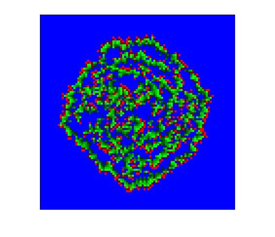
Run simulations for a few different values of the probablity (for example, 0.25, 0.5,
0.75, 1.0) and add comments to the virus.m code file about what you observe.
Part 2: Quantifying the susceptible, infected, and immune subpopulations
You now have a colorful and dynamic visualization of a spreading virus. Suppose you then want
to quantify the number of individuals who are either susceptible, infected, or immune to the
virus on each day. Add code to your virus() function to create three vectors to store
the number of susceptible individuals (value 0 in the grid), infected individuals (values 1 or 2
in the grid) or immune individuals (values 3-7 in the grid). As your simulation calculates the
state of the virus on each day, count the number of individuals in each category (you should not
need a loop for this calculation!) and store it in the appropriate vector. You can assume that
there is a total of 10,000 individuals in the population (one for each grid location). At the end
of the virus() function, plot the three populations on a single graph, with different
colors (an example is shown below).
Part 3: Modifying the initial state of the virus
With only one infected individual on the first day, these curves are not very interesting. The
final step in the construction of your program is to add the ability to specify an arbitrary
number of individuals who are infected on the first day of the simulation, and place them at
randomly selected locations of the grid. First, add a third input to the virus()
function that is used to specify the number of individuals who are infected on the first day.
Make this an optional input. If the user does not specify a value for this input, your
function should place a single infected individual at the center of grid1 at the
outset (the code currently does this). However, if the user specifies a value for this input,
place this number of 1's in grid1 at the outset. The row and column number for each
1 (infected individual) should be a random integer in the range between 2 and 99 (omit the outer
rows and columns of the grid). The built-in function randi(imax) returns a random
integer in the range from 1 to imax, and can be helpful here. (Note that the
randi() function is a relatively new addition to MATLAB and is not available in
older versions.)
The following figure is a sample plot generated by the following function call:
>> virus(100, 0.5, 10);
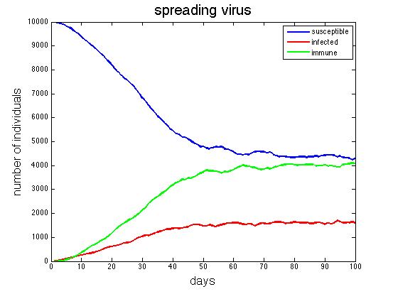
Run your simulation for 100 days, using a couple different values of the probInfect
input, combined with a couple different values for the number of individuals who are initially
infected. Add comments to your code describing how the graphs of the susceptible, infected,
and immune individuals changed with different input parameters.
How to turn in this assignment
Step 1. Complete this
online
form.
The form asks you to estimate your time spent on the problems. We
use this information to help us design assignments for future versions
of CS112. Each partner should submit their own form (it is a requirement of
completing the assignment).
Step 2. Upload your final programs to the CS server.
When you have completed all of the work for this assignment, your assign5_exercise folder
should contain one code file named ubbi.m and your assign5_problem
folder should at least contain one code file named virus.m.
Use Cyberduck to connect
to your personal account on the server and navigate to your cs112/drop/assign05 folder.
Drag your assign5_exercise and assign5_problem folders to this drop
folder. More details about this process can be found on the webpage on
Managing Assignment Work.
Step 3. Hardcopy submission.
Your hardcopy submission should include printouts of two code files:
ubbi.m and virus.m.
To save paper, you can cut and paste your two code files into one file, and you only need to
submit one hardcopy for you and your partner.
If you cannot submit your hardcopy in class on the due date, please slide
it under Ellen's office door.